Measuring the diameter of a human hair—often 40–120 μm—requires a method that doesn’t touch the sample, and that’s where diffraction helps. If you shine a laser through a strand, the light spreads out and makes a pattern of bright and dark bands on a screen. The spacing between those bands lets you work out the hair’s thickness with micrometer-level accuracy. The calculator here lets you go back and forth between hair diameter, fringe spacing, wavelength, screen distance, angular position, and maximum observable order, using the main variables as needed. Engineers and technicians use this method in lab classes, forensic fiber checks, and to keep fiber production lines in spec. Below, you'll find the core formulas, one fully worked example, essential wave optics context, and a FAQ covering real-world issues.
What is hair diffraction?
Hair diffraction describes what happens when you shine a laser at a strand of hair, and the light bends around it—creating a sequence of dark and bright stripes on a nearby wall or screen. The pattern’s dimensions are set by the hair’s thickness: measuring that lets you calculate the hair diameter, no physical contact needed.
Simple Explanation
If you picture a hair as a small obstacle in a stream, the water flows around it and makes ripples. When a laser hits a hair, light “ripples” and overlaps in a similar way, creating bright and dark stripes (fringes) on a screen. Thinner hairs cause those stripes to be farther apart. By measuring the gap between the fringes, you can figure out the hair’s thickness without needing a microscope.
📐 Browse all 1000+ Interactive Calculators
How to Use This Calculator
- Choose what you want to solve for from the dropdown. Options include hair diameter, fringe spacing, wavelength, screen distance, angular minima, and maximum observable order.
- Input your laser wavelength in nanometers and the screen distance in meters.
- Provide the measured fringe spacing (in millimeters) or hair diameter (in micrometers) depending on your goal.
- Press Calculate to get a result.
Diffraction Setup Diagram

Hair Diffraction Calculator
This calculator is intended for education, concept evaluation, and preliminary design. Results are based on the equations and assumptions described on this page, but cannot account for every real-world load case, tolerance, material property, environmental condition, installation detail, safety factor, code, or regulatory requirement. Verify all inputs, assumptions, units, and results independently before selecting components or using the result in a real application. Safety-critical, structural, medical, lifting, transportation, or regulated applications must be reviewed by a qualified engineer.
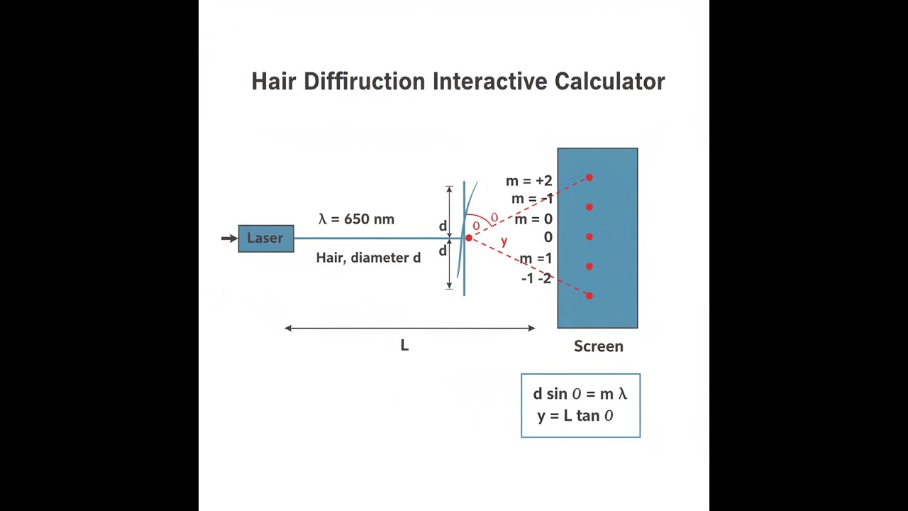
Hair Diffraction Interactive Visualizer
This animation shows how light from a laser spreads out after passing by a hair, forming alternating stripes on the other side. Adjusting the wavelength, screen distance, or hair diameter will clearly show how each one changes the spacing or sharpness of those fringes.
FRINGE SPACING
10.0 mm
ANGLE θ
0.58°
MAX ORDER
100
FIRGELLI Automations — Interactive Engineering Calculators
Governing Equations
The equation below gives you the angle at which the dark band appears, based on the hair's diameter and laser wavelength, and which “order” (fringe count from center) you’re looking at.
Single-Slit Diffraction Minimum Condition
d sin θ = m λ
d = hair diameter (slit width) [m]
θ = angular position of mth minimum [rad or degrees]
m = order number (1, 2, 3, ...) [dimensionless]
λ = wavelength of light [m]
Fringe Spacing (Small Angle Approximation)
y = (m λ L) / d
y = linear distance from central maximum to mth minimum [m]
L = distance from hair to screen [m]
Valid when θ ≪ 1 radian (typically θ < 10°), using tan θ ≈ sin θ ≈ θ
Maximum Observable Order
mmax = ⌊d / λ⌋
mmax = highest order diffraction minimum that can exist
Limited by condition sin θ ≤ 1, beyond which no physical solution exists
⌊ ⌋ denotes floor function (round down to nearest integer)
Central Maximum Width
w = (2 λ L) / d
w = full width of central bright fringe (distance between first minima on either side) [m]
Central maximum is twice as wide as subsequent maxima
Contains majority of diffracted light intensity
Simple Example
Mode: Calculate Hair Diameter from Fringe Spacing
Wavelength: 650 nm (red laser)
Screen distance: 1.0 m
Fringe spacing: 10 mm
Order number: 1
Result: d = (1 × 650×10⁻⁹ × 1.0) / 0.010 = 65 μm
Theory & Practical Applications
Physical Basis of Single-Slit Diffraction
When you shine a laser at something about the size of the wavelength—like a hair—the resulting pattern isn't a sharp shadow, but a spread of stripes and bands. Even though a hair is blocking light (not letting it through a slit), the pattern from a strand and a slit of the same width is nearly identical, except right at the center where light’s blocked (Babinet’s principle). Looking closer, every point along the hair’s width acts like a source of small ripples; the path differences cause some ripples to add up and others to cancel. The dark spots (minima) happen when the difference across the width is exactly m full wavelengths, which is why the single-slit condition is d sin θ = mλ and not the double-slit relation. For the first minimum, rays from the top and bottom edges (and points in between) combine to cause complete cancellation. Most textbook treatments miss the details on why this formula differs—zone pairing across the width is the true reason.
The main point: minima are set by the full-width path differences, not half-wavelength differences like you’d see in double-slit setups. The underlying interference works differently; that’s why the math changes.
Small Angle Approximation Validity
The formula y = mλL/d is only accurate at small angles. There are several approximations stacked up here: you assume tan θ ≈ θ and sin θ ≈ θ, both true only when θ is pretty small (less than about 10°, or 0.2 radians). At θ = 5°, your error’s still under 0.1%, but at 15°, it’s getting to 1–1.5%. Also, you’re measuring straight-line distances, ignoring any curvature from the true arc on a sphere, but unless your setup is extreme, this last factor’s negligible.
Engineers start to see errors build up past 10°, so if you want better than 5% accuracy, don’t push the small angle too far. As an example: for a 65 μm hair and a 650 nm laser at 1.5 m, the first minimum with the small angle formula is about 15 mm; the exact trig result is 14.97 mm. That’s a very small difference and fine for demos or rough checks. But climb to higher orders or wider angles and you’ll quickly lose accuracy, and the pattern starts getting too dim to spot anyway.
Wavelength Dependence and Color Effects
Because fringe spacing is proportional to wavelength, this method works for measuring light’s wavelength, not just hair thickness. Shine white light through the hair and you’ll see the different colors (wavelengths) make fringes at different places: shorter wavelengths (violet) create fringes closer together than longer ones (red). Old-school spectroscopists used known fiber diameters to eyeball unknown laser wavelengths by seeing where the fringes landed. This only works well for the first order or with a single color—higher order fringes from different colors overlap so much, everything blurs together and you can’t get clean measurements. So if you want accurate numbers, stick with monochromatic (single color) sources.
Applications in Forensic Science
Forensic techs use this approach when they can’t risk destroying or contaminating evidence. Head hair diameter depends on ethnicity and location (Asian head hair: 80–120 μm, Caucasian: 50–70 μm, African: 40–60 μm), and body hair has its own signature. With a standard HeNe laser and a meter to a screen, you’ll get noticeably different fringe spacings for thick and thin hairs—enough to distinguish most types using a simple ruler.
Of course, in crime labs, they’ll back this up with direct microscope checks and other chemical or structural tests. Diffraction stands out when you can’t touch or mount the sample. If the hair’s not perfectly round, expect the pattern to shift depending on how it’s turned. Routinely, careful labs rotate the sample and measure at several angles to get the main axes, because real-world hairs aren’t nice ideal cylinders.
Industrial Quality Control Applications
On fiber production lines, laser diffraction gauges let operators track fiber thickness in real time, right as it comes out of the extruder. When you’re running thousands of meters, even a few microns out of spec can mean a pile of wasted product or faulty spools. Systems are set up with a laser and a screen (or CCD detector) at a known gap. If the diameter drops by 3%, the fringe spacing increases by 3%, and the equipment can see this immediately. Sensors working at millisecond rates keep up with the process and allow adjustment before things drift too far.
For single filaments in the 60–80 μm range, getting ±1 μm repeatability is entirely realistic, provided the optical platform is stable and measurements are frequent enough. So, for high-volume synthetic fiber production, non-contact diffraction is far more practical than stopping the line for periodic sampling.
Worked Example: Complete Hair Measurement Procedure
Scenario: Suppose you need to confirm the diameter of a new fiber for surgical suture, specified at 73.0 μm ±3 μm. A technician sets up a 638 nm laser and a screen exactly 1.850 m away. They measure the gap from the center to the first dark fringe: 16.3 mm to the right, 16.1 mm to the left.
Part A - Calculate Fiber Diameter from Each Measurement:
Right side (y₁ = 16.3 mm = 0.0163 m):
d₁ = (1 × 638 × 10⁻⁹ × 1.850) / 0.0163 = 72.42 μm
Left side (y₂ = 16.1 mm = 0.0161 m):
d₂ = (1 × 638 × 10⁻⁹ × 1.850) / 0.0161 = 73.31 μm
Part B - Assess Measurement Quality:
Average diameter: davg = (72.42 + 73.31) / 2 = 72.87 μm
Standard deviation: σ = 0.63 μm
Uncertainty: ±2σ = 1.26 μm (95% confidence)
If left and right differ by nearly 1 μm, the fiber may be tilted or not perfectly round. Averaging both is standard practice for this sort of check.
Part C - Verify Small Angle Approximation Validity:
Using average y = 16.2 mm: tan θ = y / L = 0.0162 / 1.850 = 0.008757 θ = arctan(0.008757) = 0.5017° = 0.00876 rad sin(0.5017°) = 0.008757 So, error is 0.03%—well within what most labs would accept.
Part D - Calculate Higher Order Positions for Pattern Verification:
Second order (m = 2): y₂ = (2 × 638 × 10⁻⁹ × 1.850) / (7.287 × 10⁻⁵) = 32.4 mm
Third order (m = 3): y₃ = (3 × 638 × 10⁻⁹ × 1.850) / (7.287 × 10⁻⁵) = 48.6 mm
A technician can look for additional minima at these points. If they appear as predicted and sharp, the sample’s likely uniform and the method is working well.
Part E - Quality Control Decision:
Measured diameter: 72.87 ± 1.26 μm
Specification: 73.0 ± 3.0 μm (range: 70.0 - 76.0 μm)
So this batch passes—the process is well under control, and this non-contact method is precise enough for applications like surgical sutures, especially since it doesn’t break the sterile seal compared to using something like a micrometer.
Intensity Distribution and Fringe Visibility
The brightness of each fringe follows a sinc² ( [sin(β)/β]² ) pattern, so the central band is much brighter than the rest—over 90% of the total light is centered at zero. Only the first few fringes on each side are easily visible; the rest fade away quickly. After about four or five, they’re so dim that noise and laser bandwidth start to swamp them. Even “single” color lasers have a spread in their wavelength, so at high fringe orders, the bands begin to blur. For practical use, stick to the first few well-contrasted fringes; beyond that, getting consistent measurements is unreliable.
Frequently Asked Questions
Free Engineering Calculators
Explore our complete library of free engineering and physics calculators.
Browse All Calculators →🔗 Explore More Free Engineering Calculators
About the Author
Robbie Dickson — Chief Engineer & Founder, FIRGELLI Automations
Robbie Dickson brings over two decades of engineering expertise to FIRGELLI Automations. With a distinguished career at Rolls-Royce, BMW, and Ford, he has deep expertise in mechanical systems, actuator technology, and precision engineering.
Need to implement these calculations?
Explore the precision-engineered motion control solutions used by top engineers.


