Takt Time Production Interactive Calculator

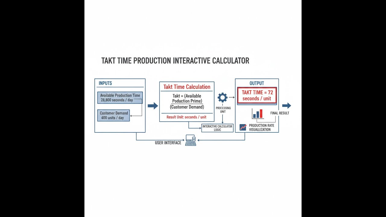
The Takt Time Production Calculator is an essential lean manufacturing tool that determines the maximum time allowed to produce one unit to meet customer demand. Used by production managers, industrial engineers, and operations teams worldwide, this calculator helps synchronize production pace with actual market requirements, eliminate waste, and optimize workforce allocation. Understanding takt time is fundamental to implementing just-in-time manufacturing, balancing production lines, and maintaining competitive delivery schedules.

📐 Browse all free engineering calculators

Visual Diagram

Takt Time Production Calculator

Takt Time Equations

Theory & Engineering Applications

Takt time, derived from the German word "Taktzeit" meaning rhythm or meter, represents one of the most fundamental concepts in lean manufacturing and production planning. Unlike cycle time, which measures how long a process actually takes, takt time defines the theoretical pace at which production must occur to satisfy customer demand exactly. This distinction is crucial: takt time is determined by external market forces (customer orders), while cycle time reflects internal process capabilities. Understanding and implementing takt time correctly transforms a production facility from push-based manufacturing—where products are made in anticipated quantities—to pull-based systems where production synchronizes precisely with consumption.

Fundamental Principles of Takt Time

The mathematical elegance of takt time belies its operational complexity. When we calculate that takt time equals available production time divided by customer demand, we are establishing a heartbeat for the entire manufacturing operation. If a facility operates 450 minutes per shift (accounting for breaks and planned maintenance) and must produce 300 units, the takt time becomes 90 seconds per unit. Every 90 seconds, one complete unit must exit the production line. This creates a powerful constraint that drives decision-making throughout the operation: any process step taking longer than 90 seconds becomes an immediate bottleneck requiring attention.

What many practitioners miss is that takt time is not merely a target—it represents the maximum permissible time per unit. Operating below takt time (faster cycle times) creates excess capacity, which can be strategically valuable for absorbing variation, conducting maintenance, or building safety stock. However, operating significantly below takt time consistently indicates overproduction waste, one of the seven deadly wastes in lean manufacturing. The optimal state maintains cycle times at approximately 85-95% of takt time, providing a buffer for normal variation while minimizing waste.

Available Time Calculation Nuances

Determining "available production time" requires careful analysis that goes beyond simply subtracting lunch breaks from shift duration. Best practice involves distinguishing between planned and unplanned downtime. Planned downtime—including scheduled breaks, shift changeovers, preventive maintenance windows, and tooling changes—should be subtracted from gross available time. Unplanned downtime from equipment failures, material shortages, or quality issues should not be subtracted when calculating takt time, because doing so disguises systemic problems and inflates the apparent pace requirement.

For example, consider a facility running two 8-hour shifts with two 15-minute breaks and one 30-minute lunch per shift. Gross time equals 960 minutes per shift. Subtracting breaks (60 minutes) and typical changeover time (20 minutes) yields 880 minutes of available production time. If this facility historically experiences 45 minutes of unplanned downtime per shift, the temptation is to calculate takt time using 835 minutes. This is incorrect. Takt time should use 880 minutes, establishing a pace target that, when met, exposes the 45 minutes of losses as waste requiring elimination through total productive maintenance (TPM) or other improvement initiatives.

Line Balancing and Workstation Distribution

Once takt time is established, production engineers face the challenge of distributing work content across workstations such that no single station exceeds the takt time limit. This process, called line balancing, directly impacts labor efficiency and production flow. The theoretical minimum number of operators equals total work content divided by takt time, but this assumes perfect distribution—rarely achievable in practice due to task interdependencies, equipment constraints, and ergonomic factors.

Line balance efficiency quantifies how closely actual distribution approaches the theoretical ideal. An efficiency of 88% indicates that 12% of available operator time is lost to imbalances—some stations finish early while waiting for the bottleneck station. In automotive assembly, world-class facilities achieve 92-95% line balance efficiency through sophisticated work allocation algorithms and continuous improvement. Lower-volume operations often accept 80-85% efficiency as economically optimal, recognizing that pursuing perfect balance has diminishing returns when changeovers are frequent.

Multi-Model Production Complexity

Real manufacturing environments rarely produce a single product at constant demand. Multi-model production lines must handle product mix variations, each with different work content and cycle time requirements. The solution involves calculating a blended takt time weighted by product mix percentages. If a line produces Model A (60% of volume, 180 seconds work content) and Model B (40% of volume, 210 seconds work content), the weighted work content is (0.60 × 180) + (0.40 × 210) = 192 seconds. This blended value informs staffing and line balance decisions more accurately than using any single product.

Advanced implementations employ heijunka (production leveling) to sequence mixed models in repeating patterns that smooth resource utilization. Rather than building all Model A units followed by all Model B units, a heijunka box might establish a sequence like A-A-B-A-B-A-A-B, distributing the higher work content of Model B evenly throughout the shift. This prevents the line from oscillating between feast and famine states, improving overall flow stability and reducing the need for excess capacity.

Worked Example: Assembly Line Design

Consider designing an assembly line for electronic control modules with the following parameters:

• Daily customer demand: 720 units
• Operating schedule: Two 7.5-hour shifts per day
• Planned breaks: 30 minutes per shift (two 15-minute breaks)
• Shift changeover: 15 minutes
• Total work content per unit: 385 seconds

Step 1: Calculate available production time per day

Gross time = 2 shifts × 7.5 hours × 60 minutes = 900 minutes
Planned downtime = 2 shifts × (30 minutes breaks + 15 minutes changeover) = 90 minutes
Available production time = 900 - 90 = 810 minutes = 48,600 seconds

Step 2: Calculate takt time

Takt time = 48,600 seconds ÷ 720 units = 67.5 seconds per unit

This means one completed unit must exit the line every 67.5 seconds to meet customer demand exactly.

Step 3: Determine theoretical number of operators

Theoretical operators = 385 seconds work content ÷ 67.5 seconds takt time = 5.70 operators

Since we cannot employ fractional operators, we round up to 6 operators.

Step 4: Calculate line balance efficiency

Line balance efficiency = 385 ÷ (6 × 67.5) × 100% = 95.1%

This indicates excellent balance with only 4.9% balance loss. Each operator theoretically handles 385 ÷ 6 = 64.2 seconds of work content on average.

Step 5: Design workstation allocation

The production engineer must now distribute 385 seconds of work across 6 stations such that no station exceeds 67.5 seconds. A possible distribution might be:

• Station 1: Component preparation and PCB loading (62 seconds)
• Station 2: Surface mount device placement (67 seconds)
• Station 3: Through-hole component insertion (65 seconds)
• Station 4: Wave soldering and cleaning (66 seconds)
• Station 5: Functional testing and calibration (63 seconds)
• Station 6: Final assembly and packaging (62 seconds)

Total = 385 seconds, with maximum station time of 67 seconds (Station 2), which is within the 67.5-second takt time. The actual line balance efficiency is 385 ÷ (6 × 67) = 95.8%, even better than theoretical because we optimized task distribution.

Step 6: Validate production capacity

Theoretical daily output = 48,600 seconds ÷ 67 seconds per unit = 725 units
This exceeds the required 720 units, providing a 0.7% capacity buffer for normal variation.

Common Implementation Pitfalls

A critical mistake involves confusing takt time with target cycle time for individual machines or processes. Takt time applies to the entire value stream—from raw material to finished good. Individual workstations within that stream may operate at different cycle times, provided the overall throughput meets takt. A stamping press might run every 15 seconds, but if each cycle produces four parts and takt time is 60 seconds per part, the press operates correctly at 25% of the line takt time.

Another frequent error is failing to update takt time when demand changes. Takt time is not static; it must be recalculated monthly, weekly, or even daily in high-variability environments. A production line designed for 90-second takt time cannot simply "run faster" if demand suddenly increases without reassessing staffing, equipment capacity, and quality systems. Similarly, when demand decreases and takt time increases, continuing to operate at the old pace generates overproduction waste.

The relationship between takt time and inventory strategy requires sophisticated understanding. Just-in-time purists advocate eliminating all buffer inventory, allowing takt time to dictate flow completely. However, practical implementations recognize that strategic buffers at decoupling points protect against variation in supplier delivery, equipment reliability, and demand fluctuation. The key is distinguishing between lean buffers (small, managed quantities at specific locations for specific reasons) and wasteful inventory (large, unmanaged accumulations hiding problems throughout the system).

Integration with Overall Equipment Effectiveness (OEE)

Takt time analysis becomes exponentially more powerful when integrated with OEE measurement. OEE captures the productivity losses from availability (downtime), performance (slow cycles), and quality (defects). When actual cycle time consistently exceeds takt time, OEE analysis pinpoints whether the root cause is equipment failures (availability), inefficient operation (performance), or rework loops (quality). This diagnostic capability transforms takt time from a planning tool into a continuous improvement driver.

For automation projects, takt time establishes the required equipment cycle time. If takt time is 45 seconds and a proposed robotic cell has a 52-second cycle time, the investment cannot meet demand without parallel cells or upstream buffering. This forces early design decisions about equipment speed, reliability requirements, and economic justification, preventing costly mistakes where automated solutions create bottlenecks rather than relieving them.

For additional production planning tools, explore the complete calculator library covering manufacturing, quality control, and operations engineering topics.

Practical Applications

Frequently Asked Questions