VSWR Voltage Standing Wave Ratio Interactive Calculator

Impedance mismatch wastes power and can damage RF transmitters, often without any obvious symptoms until you look at real numbers. This VSWR calculator gives you the reflection coefficient, return loss, mismatch loss, and percentage of reflected power based on what you already know: VSWR, impedance, or return loss. These values are important anywhere mismatch can’t be ignored—antennas, high-power transmitters, and cell bases—because even a few percent of reflected power is enough to cause problems. You’ll find formulas, a worked example, and a breakdown of standing waves and matching, plus answers to common field situations.

What is VSWR?

VSWR, or Voltage Standing Wave Ratio, is a way to see if your cable and its load are matched. VSWR of 1:1 means no reflected power—your source and load are matched. Anything higher than 1:1 means more power is coming back to the source instead of going to the antenna or load.

Simple Explanation

If you put a nozzle on a garden hose that’s the wrong size, water backs up instead of flowing freely. Mismatched impedances in an RF system do the same thing with electrical energy: some of your signal reflects back down the line, not out the antenna. VSWR tells you how bad that mismatch is—the closer to 1, the better; more delivered power, less reflected.

📐 Browse all 1000+ Interactive Calculators

How to Use This Calculator

1. Pick the calculation mode for what you know (VSWR, reflection coefficient, return loss, or impedances).
2. Type the value into the correct spot—VSWR, Γ, return loss in dB, impedance, or forward power.
3. If you’re using impedance mode, input both load impedance Z_L and line impedance Z₀ (ohms).
4. Hit Calculate to see your numbers.

System Diagram

Interactive VSWR Calculator

<> Embed this calculator → <> Embed this animation calculator →

Governing Equations

Simple Example

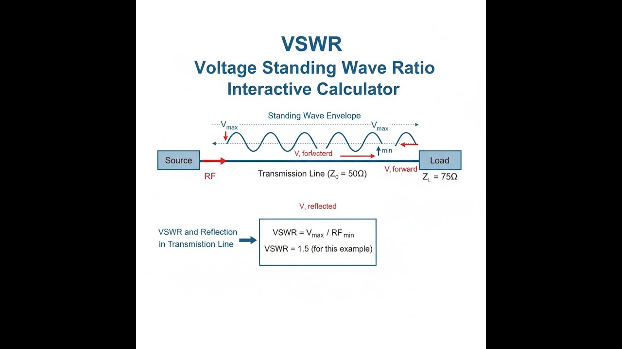
A 75Ω load connected to a 50Ω transmission line:

• Γ = (75 - 50) / (75 + 50) = 0.200
• VSWR = (1 + 0.200) / (1 - 0.200) = 1.500
• Return Loss = -20 × log₁₀(0.200) = 13.98 dB
• Reflected Power = 0.200² × 100 = 4.0%

Theory & Practical Applications of VSWR

Physical Origin of Standing Waves in Transmission Lines

Whenever the load impedance at the end of a transmission line doesn’t match the line’s characteristic impedance (Z₀), you get a reflected wave heading back toward the source. This forward-and-reflected wave combination creates stationary peaks and valleys—standing waves—along the line. VSWR is the ratio of the highest voltage to the lowest voltage along this pattern. If you have a perfect match (Z_L = Z₀), there’s no reflection and VSWR is 1. As mismatch grows, VSWR rises—if you measure 10:1, you’re reflecting over 80% of your power, which is severe.

The reflection coefficient Γ tells you what fraction of your incident voltage comes back. Its magnitude drives both VSWR and reflected power. For lossless lines, VSWR relates to |Γ| as (1 + |Γ|)/(1 - |Γ|), which just follows directly from how forward and reflected voltages add up at points of max and min. This link between VSWR and reflection coefficient is behind most RF matching calculations.

Return Loss and Its Engineering Significance

Return loss puts the mismatch into decibels, comparing how much power is reflected vs sent forward. VSWR lets you picture standing waves, but return loss is often more useful for tracking power loss. For example, 20 dB return loss means you’re reflecting about 1%—fine for standard comms, not good where transmitter reliability matters. High-power systems often want 30 dB or better (<1.07 VSWR), so only a sliver of output is reflected, reducing stress on expensive amplifiers.

Return loss and VSWR don’t scale linearly: for poor matches, a small return loss change makes big VSWR jumps; for good matches, you need to improve return loss a lot before VSWR moves more than a fraction. This is why precise instruments show return loss to hundredths of a dB, but VSWR is usually rounded to tenths. If you’re building antenna tuners, expect that getting the last couple dB of return loss improvement takes as much work as the first 20 dB.

Mismatch Loss and System Efficiency

Mismatch loss tells you how much actual power delivery drops compared to a perfect match. While return loss is about what’s reflected, mismatch loss is about system efficiency: how much less power the load gets. The formula uses (1 - |Γ|²); so a 2:1 VSWR is about 11% reflected (return loss ~9.5 dB), but this only shows up as a 0.5 dB mismatch loss—most power still gets through.

If you have several mismatches in line, their losses add up in a more complicated way than just summing dB. For example, in a cell tower setup, reflections bounce back and forth across different mismatches, so you get an infinite series of smaller reflections that don't just add up directly. Real layouts with two or three “rough” connections rarely match the sum of the individual mismatch loss values.

Impedance Matching in Antenna Systems

Antennas almost never come right at 50Ω or 75Ω, so real systems need some sort of matching network to bring VSWR down. For example, a center-fed half-wave dipole is about 73Ω—close, but still a 1.46 VSWR and nearly 2% reflected power. This can get a lot worse at band edges, with more mismatch. Practical broadband antennas need transformers, L-networks, or baluns to keep VSWR under 2:1 across the whole operating band.

With phased arrays, the impedance seen by each element swings around depending on the scan angle—what’s matched at broadside can jump to VSWR 2.5 or higher off-axis. Some advanced systems use tunable matching networks at each element, adjusting on the fly to keep VSWR low no matter where the beam is pointed. This keeps amplifiers from seeing damaging reflected power as the array scans across the sky.

VSWR Measurement Techniques and Instrumentation

Older gear relied on slotted lines or directional couplers to check VSWR, but these days, a VNA (vector network analyzer) is the gold standard, giving you both reflection magnitude and phase across frequency. VNAs measure S₁₁—the key for return loss—and convert the results to a Smith chart for easy matching visualization. They also compensate for test setup errors pretty well, so you can trust measurements up to tens of GHz if you calibrate correctly.

Field techs more often use handheld analyzers, which show VSWR or simple impedance at the cable end. Keep in mind: long, lossy cables can make the antenna VSWR look better than it really is, because reflected waves get damped out over the cable run. For example, 100 feet of common cable losing 1 dB at VHF can hide a real antenna problem by lowering observed VSWR at the transmitter—even though the mismatch is still present at the antenna end.

High-Power Transmitter Protection and VSWR Interlock Systems

Solid-state transmitters can only handle so much VSWR before they start to overheat—reflected power gets dumped into the output stage, raising its temperature quickly. For instance, 1 kW into 3:1 VSWR means 250 W comes right back; together with transmission losses, that can push output transistors well past safe limits. Modern equipment uses sensors and shutdown circuits: if the reflected-to-forward power ratio gets too high for too long, the system either cuts power or shuts down to prevent expensive damage.

The protection hardware looks at forward and reflected power using directional couplers, then calculates VSWR live. If VSWR climbs above limits, it reduces output or disables it entirely within about 50 ms. Most commercial gear will first cut power, and only go into full shutdown if the mismatch sticks around, ensuring it won’t shut down for a brief rain fade or cable wiggle.

Worked Example: Cellular Base Station Link Budget Analysis

Suppose a cell base station is rated at 20 W (43 dBm) and you’ve got a duplexer, 50 meters of 7/8" cable, and a panel antenna in the chain. Measurements show the duplexer VSWR is 1.25, and the antenna VSWR is 1.42. We’ll step through where the power goes.

Given:

• Transmitter output power: P_tx = 20W = 43.01 dBm
• Duplexer insertion loss: L_duplexer = 0.6 dB, VSWR = 1.25
• Feedline loss specification: 0.85 dB/100m at 1850 MHz for 7/8" line
• Antenna VSWR measured at antenna terminals: VSWR_ant = 1.42
• Frequency: 1850 MHz (PCS band)

Step 1: Calculate feedline loss

50 meters of cable eats up 0.425 dB.

Step 2: Calculate duplexer reflection coefficient and mismatch loss

VSWR = 1.25 gives Γ = 0.111, mismatch loss = 0.054 dB, return loss = 19.09 dB.

Step 3: Calculate antenna reflection coefficient and mismatch loss

VSWR = 1.42 gives Γ = 0.173, mismatch loss = 0.130 dB, return loss = 15.24 dB, reflected power = 2.99%.

Step 4: Calculate total system loss

Add up the numbers: total loss = 0.6 + 0.425 + 0.054 + 0.130 = 1.209 dB.

Step 5: Calculate delivered power to antenna

P_delivered = 43.01 dBm - 1.209 dB = 41.80 dBm = 15.14 W

Step 6: Calculate radiated power accounting for antenna reflection

P_radiated = 15.14 W × (1 - 0.173²) = 14.69 W
Reflected power = 15.14 W × 0.173² = 0.45 W

Results interpretation: Of the 20 W output, about 21% is lost to normal component/cable loss and another 4% to mismatch. You’ll actually radiate about 14.7 W. Some reflected power burns off in the cable; some bounces back toward the transmitter. For most cell sites, these losses are tolerable—low VSWR does help, especially if you’re close to coverage limits or pushing your amplifiers near their thermal ceiling.

VSWR in Non-50Ω Systems and Impedance Standards

Most RF work uses 50Ω lines (good power handling vs loss), but TV and video prefer 75Ω for cable specs. The VSWR formulas stay the same no matter the reference impedance, but if you mix 50Ω and 75Ω gear, you’re going to have mismatch—sometimes VSWR over 1.5 even with a perfectly matched antenna—just because the transmitter “sees” the wrong impedance at the cable input.

Lab gear and RF connectors are usually spec’d tightly—high-quality parts keep VSWR under 1.2—so test uncertainty stays low. To go from 50Ω to 75Ω with less mismatch, you can use a quarter-wave transformer section. For example, a 61.2Ω section of coax (√(50×75)) about 37.5 mm long at 1 GHz (assuming PTFE dielectric) will keep VSWR under 1.1 over a reasonable bandwidth.

Frequently Asked Questions

Video Walkthrough - How to Use This Calculator