Estimating how fast water moves through soil is a critical first step in dozens of engineering scenarios — excavation dewatering, aquifer characterization, drainage layer design, and contaminant plume modeling all depend on getting hydraulic conductivity right before you commit to a design. Use this Permeability Grain Size Calculator to calculate hydraulic conductivity (permeability) from grain size characteristics using empirical methods including the Hazen, Kozeny-Carman, Breyer, Slichter, and Terzaghi equations. It matters across geotechnical, environmental, and civil engineering — anywhere granular soil controls water movement. This page covers the formulas, a worked example, the underlying theory, and a FAQ.
What is soil permeability from grain size?
Soil permeability (hydraulic conductivity) is a measure of how easily water flows through soil. Grain size calculators estimate it from particle size data — specifically the effective grain diameter — without needing a full lab permeability test.
Simple Explanation
Think of soil like a pile of marbles. Bigger marbles leave bigger gaps between them, so water flows through quickly. Smaller grains pack tighter, leaving tiny gaps that slow water down. Grain size calculators use that relationship — bigger particles mean higher permeability — to give you a fast, practical estimate.
📐 Browse all 1000+ Interactive Calculators
Diagram

How to Use This Calculator
- Select your calculation method from the Calculation Mode dropdown — Hazen, Kozeny-Carman, Breyer, Slichter, Terzaghi, or Reverse.
- Enter your effective grain size D₁₀ in millimetres (and porosity or void ratio if your chosen method requires them).
- Enter the field water temperature in °C so the calculator can apply the viscosity correction.
- Click Calculate to see your result.
Permeability Grain Size Calculator
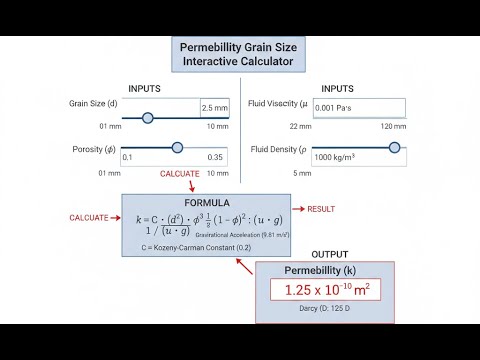
Permeability Grain Size Interactive Visualizer
Watch how soil grain size directly controls water flow through visualizing the relationship between particle diameter and hydraulic conductivity. Adjust the effective grain size to see real-time permeability changes across multiple empirical equations.
HAZEN k (cm/s)
2.3×10⁻³
KOZENY-CARMAN
1.8×10⁻³
CLASSIFICATION
MED SAND
FIRGELLI Automations — Interactive Engineering Calculators
Equations & Variables
Use the formula below to calculate hydraulic conductivity from effective grain size using the Hazen equation.
Hazen Equation (1892)
k = C · D₁₀²
Where:
- k = hydraulic conductivity (permeability) at 20°C (cm/s)
- C = Hazen coefficient (typically 1.0 for cm/s when D₁₀ in cm, or 0.01 when D₁₀ in mm)
- D₁₀ = effective grain size, 10% passing diameter (mm)
Valid for uniformly graded fine to medium sands with D₁₀ between 0.1 and 3.0 mm and uniformity coefficient Cu less than 5.
Use the formula below to calculate hydraulic conductivity accounting for porosity using the Kozeny-Carman equation.
Kozeny-Carman Equation
k = (D₁₀² · n³) / (180 · (1 - n)²)
Where:
- k = hydraulic conductivity (cm/s)
- D₁₀ = effective grain size (cm)
- n = porosity (dimensionless, 0 to 1)
Theoretical derivation based on flow through idealized porous media; applicable across wider range of soil types when porosity is known.
Use the formula below to calculate hydraulic conductivity using the Breyer equation.
Breyer Equation
k = 0.0060 · D₁₀²
Where:
- k = hydraulic conductivity (cm/s)
- D₁₀ = effective grain size (cm)
- 0.0060 = empirical Breyer coefficient
Use the formula below to calculate the field permeability from the standardised 20°C value using the temperature correction.
Temperature Correction
kT = k₂₀ · (μ₂₀ / μT)
Where:
- kT = permeability at field temperature T (cm/s)
- k₂₀ = permeability at standard 20°C (cm/s)
- μ₂₀ = dynamic viscosity of water at 20°C
- μT = dynamic viscosity at temperature T
Simplified empirical approximation: viscosity ratio → (1 + 0.0337T + 0.000221T²) / (1 + 0.0337·20 + 0.000221·20²)
Simple Example
Using the Hazen equation for a clean medium sand:
- D₁₀ = 0.3 mm, temperature = 20°C
- k₂₀ = 0.01 × (0.3)² = 0.01 × 0.09 = 0.0009 cm/s
- Uniformity coefficient Cu = 2.8 — within Hazen's valid range
- Result: k₂₀ = 9.0 × 10⁻⁴ cm/s — classified as fine sand with good drainage
Theory & Engineering Applications
Fundamental Relationship Between Grain Size and Permeability
The hydraulic conductivity (permeability) of granular soils is fundamentally controlled by the void space geometry, which in turn is primarily determined by grain size distribution. Allen Hazen's pioneering 1892 work established the empirical relationship between the effective grain size D₁₀ and permeability for clean, uniformly graded sands. His research, conducted during the development of rapid sand filters for water supply systems in Massachusetts, demonstrated that permeability is proportional to the square of the effective grain diameter. This quadratic relationship arises from the physics of laminar flow through porous media, where both flow area and hydraulic radius scale with grain size.
The D₁₀ parameter represents the grain diameter at which 10% (by weight) of the soil particles are finer. This metric proved more reliable than mean grain size because it characterizes the smallest pore throats that dominate flow resistance. A soil with D₁₀ = 0.25 mm contains particles where 10% pass through a 0.25 mm sieve opening. Hazen's original coefficient was calibrated for filter sands with temperatures near 10°C, but modern practice standardizes to 20°C and applies temperature corrections based on water viscosity changes.
Limitations and Non-Obvious Considerations
While widely used for preliminary estimates, grain-size-based permeability equations have significant limitations that practitioners must understand. The Hazen equation loses accuracy for soils with uniformity coefficients (Cu = D₆₀/D₁₀) exceeding 5, where well-graded particle distributions create complex pore structures. In such cases, fine particles can infiltrate voids between coarser grains, drastically reducing permeability beyond what grain size alone would predict. A soil with D₁₀ = 0.3 mm but Cu = 15 may exhibit permeability an order of magnitude lower than Hazen's equation would suggest.
The presence of even small amounts of fines (silt and clay) dramatically affects permeability in ways not captured by D₁₀ alone. Research by Chapuis and Aubertin demonstrated that as little as 5-7% fines content can reduce permeability by 50% compared to clean sand predictions. This occurs because fine particles coat grain surfaces, bridge pore throats, and increase tortuosity of flow paths. Field permeability often measures 2-10 times lower than laboratory predictions for this reason, as natural soils rarely match the ideal clean, uniform conditions under which empirical equations were developed.
Fabric and structure—the spatial arrangement of particles—introduce another layer of complexity. Soils deposited by flowing water develop horizontal laminations and preferred grain orientations that create anisotropic permeability, with horizontal conductivity often 2-5 times greater than vertical. Compaction energy and method significantly alter pore structure even while preserving the same grain size distribution and density. A vibratory-compacted sand may show 40% higher permeability than the same sand compacted by kneading, despite identical D₁₀ values.
Engineering Applications Across Multiple Disciplines
Geotechnical engineers employ permeability-grain size relationships during site investigation planning and preliminary design phases. When drilling logs reveal sandy strata, grain size analysis from disturbed samples enables rapid permeability estimation before conducting expensive in-situ permeability tests or installing piezometers. This accelerates conceptual foundation design, allowing engineers to identify whether dewatering will be necessary for excavation, estimate pumping rates for initial equipment sizing, and assess consolidation settlement timeframes for clay layers beneath granular strata. A foundation excavation in sand with calculated k = 0.08 cm/s would require continuous pumping at approximately 150-300 gallons per minute per 100 feet of trench, fundamentally different from sand with k = 0.003 cm/s where seepage control might be achieved with sump pumping alone.
Environmental engineers and hydrogeologists utilize these calculations for groundwater flow modeling and contaminant transport analysis. When characterizing aquifer materials for remediation projects, grain size distribution from soil borings provides the first estimate of hydraulic conductivity for flow net construction and capture zone analysis. The relationship between grain size and permeability helps explain why contaminant plumes preferentially migrate through coarser sediment layers. A contaminated site with interbedded silty sand (D₁₀ = 0.08 mm, k ≈ 6×10⁻⁴ cm/s) and medium sand (D₁₀ = 0.4 mm, k ≈ 0.016 cm/s) will exhibit channelized flow with 95% of groundwater flux through the coarser unit despite it comprising only 40% of aquifer thickness.
Pavement engineers apply permeability-grain size relationships when designing drainage layers and open-graded friction courses. The California Department of Transportation specifies minimum D₁₀ values for base course materials to ensure adequate drainage capacity beneath pavements. A permeable base specification requiring k ≥ 0.35 cm/s translates to D₁₀ ≥ 0.6 mm for clean, uniformly graded material. This prevents pore pressure buildup during freeze-thaw cycles and extends pavement service life by rapidly removing infiltrating water.
Worked Example: Dewatering Design for Foundation Excavation
A construction project requires excavation to 4.2 meters below grade for a building foundation in an urban area. Geotechnical investigation reveals the following soil profile: 0-1.5 m sandy silt fill, 1.5-6.0 m medium-dense sand, below 6.0 m dense silty sand. Groundwater table encountered at 2.8 m depth. Sieve analysis of the medium sand layer shows D₁₀ = 0.31 mm, D₃₀ = 0.58 mm, D₆₀ = 0.89 mm. The contractor needs to estimate pumping requirements for excavation dewatering. Measured groundwater temperature is 14°C.
Step 1: Calculate uniformity coefficient
Cu = D₆₀ / D₁₀ = 0.89 mm / 0.31 mm = 2.87
Since Cu is less than 5, Hazen equation is applicable.
Step 2: Apply Hazen equation for k at 20°C
k₂₀ = 0.01 × D₁₀² = 0.01 × (0.31)² = 0.01 × 0.0961 = 0.000961 cm/s
Step 3: Apply temperature correction for field conditions at 14°C
Viscosity ratio = (1 + 0.0337×14 + 0.000221×14²) / (1 + 0.0337×20 + 0.000221×20²)
Viscosity ratio = (1 + 0.472 + 0.043) / (1 + 0.674 + 0.088) = 1.515 / 1.762 = 0.860
k₁₄ = k₂₀ × 0.860 = 0.000961 × 0.860 = 0.000827 cm/s
Step 4: Convert to practical units and assess drainage characteristics
k₁₄ = 0.000827 cm/s = 8.27×10⁻⁴ cm/s = 0.714 m/day = 2.61×10⁻⁵ ft/s
This permeability indicates fair to good drainage. The sand will allow water movement but requires active dewatering.
Step 5: Estimate seepage rate using simplified approach
For a rectangular excavation 18m × 24m with drawdown of 1.5m (lowering GWT from 2.8m to 4.3m, below excavation base):
Using simplified radial flow assumption for preliminary estimate:
Q ≈ k × π × d × (H² - h²) / ln(R/rw)
Where d = aquifer thickness (3.2m from water table to bottom of permeable layer), H = initial head (3.2m), h = drawdown head (1.7m), R = radius of influence (approximately 50m for this drawdown), rw = equivalent well radius (≈8m for rectangular excavation)
Q ≈ (0.000827 cm/s) × π × (320 cm) × ((320)² - (170)²) / ln(5000/800)
Q ≈ 0.000827 × 3.142 × 320 × (102,400 - 28,900) / 1.833
Q ≈ 0.000827 × 3.142 × 320 × 73,500 / 1.833 = 33,100 cm³/s = 0.0331 m³/s = 524 gallons per minute
Engineering implications: The calculated permeability of 8.27×10⁻⁴ cm/s confirms that wellpoint dewatering or deep wells will be necessary. The estimated 524 gpm flow rate requires specification of pumps with at least 650 gpm capacity (allowing 25% safety factor). This rate suggests 3-4 wellpoints around the excavation perimeter with individual pump capacities of 150-175 gpm each. The relatively low permeability also indicates that drawdown will require 24-48 hours to achieve design levels before excavation can safely begin. If actual field testing reveals 30% fines content not apparent from D₁₀ analysis, actual permeability could be 40-60% lower, requiring pump capacity adjustments and longer drawdown periods. This example demonstrates why grain-size estimates guide preliminary planning but must be verified with pumping tests before final dewatering system design.
Advanced Considerations for Practitioners
Modern geotechnical practice recognizes that simple grain-size correlations represent only the starting point for permeability assessment. Site-specific calibration against field permeability tests (slug tests, pumping tests, or piezometer monitoring) allows engineers to develop correction factors accounting for local conditions. Documentation of such factors builds institutional knowledge—for example, a consulting firm working repeatedly in glacial till deposits might determine that local materials consistently exhibit permeability 30% lower than Hazen predictions, leading to refined regional correlations.
For more comprehensive resources on geotechnical engineering calculations and analysis tools, visit the engineering calculator library.
Practical Applications
Scenario: Municipal Water Treatment Plant Filter Design
Jennifer, a water resources engineer designing a rapid sand filter for a municipal treatment plant expansion, needs to select appropriate filter media. The design calls for an effective size (D₁₀) that will provide hydraulic conductivity between 0.02 and 0.05 cm/s to achieve target filtration rates while preventing excessive head loss. Using the Hazen equation, she calculates that sand with D₁₀ = 0.45 mm will yield k = 0.0020 cm/s at 20°C. However, actual filtration occurs at approximately 12°C during winter months, so she applies the temperature correction factor of 0.82, resulting in k₁₂ = 0.0164 cm/s—well within specifications. She also verifies that the sand supplier can consistently deliver material with uniformity coefficient Cu less than 1.7 to maintain Hazen equation validity. This preliminary calculation allows her to specify procurement requirements and confirm feasibility before conducting pilot-scale testing, saving three weeks in the design schedule and enabling timely bidding for the $2.3 million filter construction contract.
Scenario: Environmental Remediation Site Assessment
Marcus, an environmental consultant investigating petroleum contamination at a former service station, receives soil boring logs showing the shallow aquifer consists primarily of fine to medium sand. Laboratory sieve analysis of samples from the saturated zone reveals D₁₀ = 0.18 mm with Cu = 3.2. Using the permeability grain size calculator with the Hazen equation, he estimates hydraulic conductivity of approximately 0.0032 cm/s. This value is critical for modeling contaminant plume migration and designing a pump-and-treat remediation system. The calculated permeability indicates the aquifer has fair drainage characteristics—sufficient to extract groundwater for treatment but requiring careful well spacing to maintain hydraulic control. Based on this estimate, Marcus proposes installing five extraction wells in a line downgradient of the source area, each capable of pumping 15-20 gallons per minute. The permeability calculation helps him prepare a defensible remedial action plan for regulatory approval and provides the basis for estimating that remediation will require 3-4 years to reduce dissolved hydrocarbon concentrations below cleanup standards, setting realistic expectations for his client's environmental liability timeline.
Scenario: Sports Field Drainage System Design
David, a landscape architect designing a professional soccer training facility, must specify drainage aggregate materials to keep the field playable within 2 hours after heavy rainfall. Local building codes require subsurface drainage systems to have minimum permeability of 0.15 cm/s. He uses the reverse calculation mode to determine that achieving this performance requires drainage stone with D₁₀ of at least 1.23 mm. Cross-referencing with ASTM C33 aggregate gradation specifications, he selects No. 57 stone (crushed aggregate ranging from 19 mm to 4.75 mm) which typically has D₁₀ values of 5-8 mm—providing substantial safety margin above the minimum requirement. The calculator also helps him evaluate a cost-saving alternative: using coarser sand (D₁₀ = 0.95 mm) for a shallow drainage blanket beneath the rootzone, which yields k = 0.090 cm/s using the Hazen equation. While slightly below the strict code requirement, this permeability is adequate for the shallow blanket layer when combined with the stone-filled drainage trenches. His calculations, documented in construction drawings, satisfy the geotechnical engineer's review and allow the contractor to source materials locally rather than importing premium drainage aggregates, reducing material costs by $18,000 while maintaining full drainage functionality for the $850,000 field construction project.
Frequently Asked Questions
Why does the Hazen equation only work for certain soil types? +
How significant is temperature correction in practical applications? +
What's the difference between permeability and hydraulic conductivity? +
Why do field permeability tests often give lower values than grain-size predictions? +
Can I use these equations for gravel or for clay soils? +
How does compaction affect permeability compared to grain-size predictions? +
Free Engineering Calculators
Explore our complete library of free engineering and physics calculators.
Browse All Calculators →🔗 Explore More Free Engineering Calculators
About the Author
Robbie Dickson — Chief Engineer & Founder, FIRGELLI Automations
Robbie Dickson brings over two decades of engineering expertise to FIRGELLI Automations. With a distinguished career at Rolls-Royce, BMW, and Ford, he has deep expertise in mechanical systems, actuator technology, and precision engineering.
Need to implement these calculations?
Explore the precision-engineered motion control solutions used by top engineers.


