Depth Of Field Interactive Calculator

The Depth of Field (DoF) calculator is an essential optical engineering tool that determines the distance range in which objects appear acceptably sharp in an image. Used by photographers, lens designers, machine vision engineers, and optical system developers, this calculator computes near and far focus limits, total depth of field, and hyperfocal distance based on focal length, aperture, sensor size, and subject distance. Understanding depth of field is critical for optimizing image quality in applications ranging from industrial inspection systems to cinematography and scientific microscopy.

📐 Browse all free engineering calculators

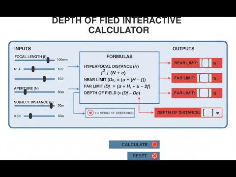
System Diagram

Depth of Field Interactive Calculator

Governing Equations

Theory & Engineering Applications

Depth of field represents one of the most fundamental concepts in optical engineering, defining the distance range over which objects appear acceptably sharp when imaged through a lens system. Unlike the idealized thin lens equation that predicts a single focal plane, real optical systems produce a gradual transition from sharp to blurred as objects move away from the exact focus distance. The boundaries of acceptable sharpness are defined by the circle of confusion—a critical parameter that depends on sensor characteristics, viewing conditions, and human visual perception limits.

The Physics of Defocus and Circle of Confusion

When a point source is imaged by a lens, the geometrical optics predict that light converges to a perfect point at the focal plane. However, at distances other than the exact focus position, the converging cone of light intersects the sensor plane as a circular disk rather than a point. The diameter of this blur circle grows linearly with the distance from the focused plane. The circle of confusion criterion establishes the maximum acceptable blur diameter—typically 1/1500 of the sensor width for photographic applications, though this value varies significantly based on final image size, viewing distance, and required resolution.

The conventional CoC formula (c = sensor_width / 1500) originates from film-era photography standards where an 8×10 inch print viewed at 10 inches would not reveal blur in circles smaller than about 0.2mm at the viewing distance. For a 35mm full-frame sensor (36mm width), this yields c ≈ 0.024mm. However, modern high-resolution sensors and digital viewing at 100% magnification often require stricter criteria—some engineers use divisors of 2000 or even 2500 for critical applications like machine vision inspection systems.

Hyperfocal Distance and Optimization Strategies

The hyperfocal distance represents a critical optimization point in optical system design. When a lens is focused at the hyperfocal distance H, the depth of field extends from H/2 to infinity—maximizing the total in-focus range. This property makes hyperfocal focusing essential in applications requiring maximum depth coverage, such as landscape photography, architectural documentation, and fixed-focus surveillance systems.

The hyperfocal distance H = f²/(N·c) + f reveals several non-intuitive relationships. The quadratic dependence on focal length means that doubling the focal length quadruples the hyperfocal distance, dramatically reducing depth of field for telephoto lenses. The inverse relationship with aperture number means that stopping down (increasing N) reduces the hyperfocal distance proportionally, extending depth of field. However, diffraction effects impose practical limits—beyond approximately f/16, diffraction-induced resolution loss may exceed the depth of field benefits from smaller apertures.

Asymmetric Depth Distribution

A frequently misunderstood aspect of depth of field is its asymmetric distribution around the focus plane. For subjects closer than the hyperfocal distance, depth of field extends approximately one-third in front of the focus point and two-thirds behind it. This 1:2 ratio is not exact and varies with subject distance—approaching 1:1 for extreme close-up work and becoming more asymmetric as the subject approaches the hyperfocal distance.

The mathematical basis for this asymmetry lies in the hyperbolic nature of the near and far limit equations. As subject distance s approaches the hyperfocal distance H, the denominator (H - s) in the far limit equation approaches zero, causing the far limit to extend toward infinity much faster than the near limit approaches the lens. This behavior has significant practical implications for focus stacking in macro photography and scene depth planning in cinematography.

Machine Vision and Industrial Applications

In machine vision systems, depth of field calculations must account for factors beyond traditional photography. Industrial inspection systems often require the entire target object to fall within the depth of field simultaneously while maintaining resolution sufficient to detect defects as small as 0.1mm. This creates a challenging optimization problem: achieving maximum depth of field typically requires small apertures, but small apertures reduce light throughput and may introduce diffraction that degrades resolution.

Engineers frequently employ telecentric lens designs in machine vision to address depth of field limitations. Telecentric lenses maintain constant magnification across the depth of field range, eliminating perspective errors and enabling accurate dimensional measurements of objects at varying distances within the field of view. The trade-off is reduced working distance and larger, more expensive lens assemblies. For a typical telecentric lens with 0.1× magnification imaging a 50mm field of view, the depth of field at f/8 might extend 12-15mm—adequate for most industrial parts inspection.

Cinematography and Bokeh Control

In cinematography, precise depth of field control serves as a powerful storytelling tool, directing viewer attention through selective focus. Cinema cameras with large Super35 (24.6mm width) or full-frame sensors enable shallow depth of field looks that were impossible with smaller video formats. A 50mm lens at f/1.4 focused on a subject 2 meters away produces a total depth of field of only 77mm on a full-frame sensor—creating strong subject isolation and smooth background blur (bokeh).

The aesthetic quality of out-of-focus regions depends on aperture blade count and shape. Lenses with more aperture blades (9-11 blades) produce rounder bokeh circles, while fewer blades create polygonal highlights. Spherical aberration also affects bokeh appearance—undercorrected lenses create "soap bubble" effects with bright edges around blur circles, while overcorrected designs concentrate light in the center. High-end cinema lenses are specifically designed to control these characteristics, with some manufacturers offering custom aperture blade designs for distinctive bokeh signatures.

Worked Example: Portrait Photography System Design

Consider a professional portrait photographer designing an optical system to achieve pleasing subject isolation. The requirements are: full-frame sensor (36mm width), 85mm focal length, subject distance 3.0 meters, and maximum tolerable background blur that keeps features at 5.0 meters completely out of focus while maintaining sharp focus on the subject's face (±150mm depth).

Step 1: Calculate circle of confusion
c = 36 / 1500 = 0.024 mm

Step 2: Determine required depth of field
Target DoF = 2 × 150mm = 300mm = 0.3 m
The subject's face should remain sharp across ±150mm from the focus point.

Step 3: Calculate required aperture
We need to solve for N given f = 85mm, s = 3000mm, target DoF = 300mm, c = 0.024mm.

Using the complete depth of field equation derived from near and far limits:
DoF ≈ (2 × N × c × s²) / (f² - N × c × s)
For cases where s is much larger than f, which applies here.

Rearranging for N:
300 = (2 × N × 0.024 × 3000²) / (85² - N × 0.024 × 3000)
300 × (7225 - 72N) = 432000N
2167500 - 21600N = 432000N
2167500 = 453600N
N = 4.78

The photographer should use approximately f/4.8 (practically f/4.5 or f/5.0).

Step 4: Calculate actual depth of field at f/5.0
H = (85² / (5.0 × 0.024)) + 85 = 60208 + 85 = 60293mm = 60.3m

D_n = (3000 × 60293) / (60293 + 3000) = 180879000 / 63293 = 2858mm = 2.858m

D_f = (3000 × 60293) / (60293 - 3000) = 180879000 / 57293 = 3157mm = 3.157m

Total DoF = 3157 - 2858 = 299mm ≈ 0.3m ✓

Step 5: Verify background blur at 5.0m
At 5000mm distance, the blur circle diameter can be estimated:
Blur diameter = (|5000 - 3000| / 3000) × (f / N) × aperture_factor
≈ (2000 / 3000) × (85 / 5.0) × 0.667 = 0.667 × 17 × 0.667 ≈ 7.6mm

This creates substantial background blur (7.6mm circle of confusion versus the 0.024mm acceptance criterion—approximately 316× larger), ensuring complete defocusing of background elements. The system meets both sharpness and aesthetic isolation requirements.

Practical considerations: At f/5.0, diffraction effects remain negligible (Airy disk diameter ≈ 0.0067mm, well below the CoC limit). Light throughput is adequate for outdoor portraits or studio lighting. The 299mm depth of field provides sufficient tolerance for subject movement during a photo session while maintaining facial feature sharpness across typical head depth (approximately 200-250mm from nose to ears).

This example demonstrates how depth of field calculations enable precise engineering of optical systems to meet both technical specifications and aesthetic requirements. Professional cinematographers and photographers routinely perform these calculations to select optimal focal length, aperture, and working distance combinations for specific creative and technical objectives.

For additional optical engineering calculations and resources, visit the FIRGELLI engineering calculator library.

Practical Applications

Frequently Asked Questions