Getting the maximum usable depth of field out of a lens isn't guesswork — it requires knowing the exact focus distance where everything from a near point to infinity lands within acceptable sharpness. Use this Hyperfocal Distance Calculator to calculate hyperfocal distance, near and far depth of field limits, total DoF, required aperture, or back-calculated focal length using focal length, f-number, circle of confusion, and focus distance. It matters across landscape photography, machine vision, aerial reconnaissance, autonomous vehicle cameras, and any system where fixed-focus operation must cover a defined depth range. This page covers the full formula set, a worked example, the underlying optical theory, and a practical FAQ.
What is hyperfocal distance?
Hyperfocal distance is the closest focus point at which a lens keeps everything from that distance all the way to infinity acceptably sharp. Focus your lens at exactly this distance and you get the maximum possible depth of field for your chosen focal length, aperture, and sensor size.
Simple Explanation
Think of it like a spotlight beam — you can spread it wide or keep it narrow. Hyperfocal distance is the trick that spreads your camera's sharp zone as wide as physically possible. Set your focus at that one magic distance and your camera treats everything from halfway to that point, all the way out to the horizon, as sharp. It's not a trick — it's just geometry working in your favour.
📐 Browse all 1000+ Interactive Calculators
Table of Contents
How to Use This Calculator
- Select your calculation mode from the dropdown — hyperfocal distance, near/far DoF limit, total DoF, required aperture, or focal length from hyperfocal.
- Enter your lens focal length in mm, aperture f-number, and circle of confusion in mm. Add focus distance or hyperfocal distance if your selected mode requires them.
- Not sure on values? Hit Try Example to load a working 50mm f/8 full-frame scenario automatically.
- Click Calculate to see your result.
Simple Example
Inputs: Focal length = 50 mm, Aperture = f/8, Circle of confusion = 0.03 mm
Formula: H = f² / (N × c) + f
Result: H = (50²) / (8 × 0.03) + 50 = 2500 / 0.24 + 50 ≈ 10,467 mm = 10.47 m
Focus at 10.47 m and everything from 5.23 m to infinity is acceptably sharp.
Optical Diagram

Hyperfocal Distance Interactive Calculator
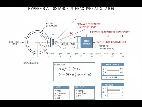
Hyperfocal Distance Interactive Visualizer
Watch how focal length, aperture, and circle of confusion affect your depth of field coverage. Focus at the hyperfocal distance to maximize sharpness from half that distance to infinity.
HYPERFOCAL
17.4 m
NEAR LIMIT
8.7 m
FAR LIMIT
∞
TOTAL DOF
∞
FIRGELLI Automations — Interactive Engineering Calculators
Equations & Variables
Use the formula below to calculate hyperfocal distance.
Hyperfocal Distance (Classic Formula)
H = Hyperfocal distance (mm or m depending on units)
f = Focal length of the lens (mm)
N = Aperture f-number (dimensionless)
c = Circle of confusion diameter (mm)
Use the formula below to calculate the near depth of field limit.
Near Depth of Field Limit
Dn = Near limit of acceptable sharpness (mm or m)
s = Focus distance from lens (mm or m)
H = Hyperfocal distance (same units as s)
f = Focal length (same units as s)
Use the formula below to calculate the far depth of field limit.
Far Depth of Field Limit
Df = Far limit of acceptable sharpness (mm or m)
Note: When s ≥ H, the far limit extends to infinity (∞)
Condition: Formula valid only when H - s + f > 0
Use the formula below to calculate total depth of field.
Total Depth of Field
DoF = Total depth of field (mm or m)
Maximum DoF: Achieved when focusing exactly at hyperfocal distance
Range: Extends from H/2 to infinity when focused at H
Theory & Engineering Applications
Fundamental Optical Principles of Hyperfocal Distance
Hyperfocal distance represents the focusing distance that maximizes depth of field for a given optical configuration, creating acceptable sharpness from half the hyperfocal distance to infinity. This principle derives from geometrical optics and the physical behavior of light diffraction through finite apertures. When a lens focuses at the hyperfocal distance, points at infinity project onto the image sensor with a circle of confusion exactly equal to the maximum acceptable blur circle, while the near limit occurs at precisely half the hyperfocal distance. This relationship is not arbitrary but emerges from the symmetric properties of the thin lens equation and the geometry of converging light cones.
The circle of confusion (CoC) parameter is critical and often misunderstood. It represents the maximum diameter of a blur spot that the human eye perceives as acceptably sharp when viewing an image under standard conditions. For 35mm full-frame sensors, a CoC of 0.030 mm is conventional, derived from viewing an 8×10 inch print at 25 cm distance. However, modern high-resolution sensors and large display formats demand smaller CoC values—often 0.020 mm or even 0.015 mm for critical work. Sensor crop factors directly affect CoC selection: an APS-C sensor (1.5× crop) uses approximately 0.020 mm, while Micro Four Thirds (2× crop) uses 0.015 mm. Failing to account for sensor size leads to incorrect hyperfocal calculations and suboptimal depth of field control.
Practical Limitations and Non-Ideal Behaviors
A critical but often overlooked limitation is that hyperfocal distance formulas assume thin lens approximations and geometric optics, which break down at very small apertures where diffraction becomes dominant. Beyond approximately f/16 on full-frame sensors, diffraction softening begins to exceed the benefits of increased depth of field, creating what photographers call the "diffraction limit." The Airy disk diameter d = 2.44 × λ × N (where λ is wavelength, approximately 550 nm for visible light) grows linearly with f-number. At f/22, the Airy disk diameter reaches 0.030 mm—matching typical CoC values and indicating that diffraction, not geometric blur, now limits resolution. Therefore, blindly stopping down to f/32 for maximum depth of field often produces softer overall images than shooting at f/11 with focus stacking techniques.
Lens breathing and focus shift further complicate practical hyperfocal distance applications. Many modern autofocus lenses change effective focal length as focus distance varies—a 50mm lens might measure 48mm at infinity and 52mm at close focus. This 8% variation directly affects hyperfocal distance calculations, creating discrepancies between theoretical and actual depth of field. Additionally, some lens designs exhibit longitudinal chromatic aberration that shifts the plane of best focus for different wavelengths, meaning that while the geometric focus may be optimal, color fringing can reduce perceived sharpness at depth of field boundaries.
Engineering Applications Across Industries
In aerial and satellite reconnaissance systems, hyperfocal distance calculations determine optimal sensor configurations for maximum ground coverage with acceptable resolution. A reconnaissance aircraft flying at 3000 meters altitude using a 150mm focal length lens at f/8 with a 0.012 mm CoC (accounting for high-resolution CCD sensors) achieves a hyperfocal distance of 15,625 meters. Focusing at this distance ensures sharp imagery from 7,812 meters to infinity, covering the ground and distant horizon simultaneously. Mission planners use these calculations to balance altitude, lens selection, and aperture settings for optimal intelligence gathering.
Machine vision systems in industrial quality control rely on hyperfocal principles when inspecting three-dimensional objects on conveyor belts. A typical system uses a 25mm lens at f/5.6 with a 0.008 mm CoC (matching 1-inch format sensors with 5-megapixel resolution). The resulting hyperfocal distance of 13.8 meters allows inspection cameras mounted above conveyors to maintain focus on parts varying in height by ±3 meters while traveling at conveyor speeds up to 2 meters per second. This eliminates the need for expensive autofocus systems or multiple fixed-focus cameras at different heights.
Autonomous vehicle perception systems apply modified hyperfocal concepts to stereo vision and LIDAR fusion. Forward-facing cameras use 6mm focal lengths at f/4 with 0.006 mm CoC, yielding hyperfocal distances around 2.25 meters. This ensures pedestrians at 1.5 meters and traffic signals at 100 meters both fall within the depth of field, critical for simultaneous near-field obstacle detection and far-field scene understanding. The computational burden of continuous autofocus would introduce unacceptable latency in real-time decision systems, making fixed hyperfocal focusing the preferred approach.
Worked Example: Landscape Photography System Design
A landscape photographer plans to shoot in Yosemite Valley using a full-frame DSLR with a 24mm wide-angle lens. The scene includes foreground boulders 3.5 meters from the camera and distant granite walls extending to the visual horizon. The photographer must determine the optimal aperture and focus distance to ensure the entire scene remains acceptably sharp when printed at 16×24 inches and viewed at 50 cm distance.
Step 1: Determine Circle of Confusion
For critical landscape work with large prints, use CoC = 0.020 mm rather than the standard 0.030 mm. This accounts for modern high-resolution sensors (24+ megapixels) and critical viewing conditions.
Step 2: Select Initial Aperture
Choose f/11 as a starting point—small enough for substantial depth of field but large enough to avoid significant diffraction effects on full-frame sensors. We'll verify this choice produces the required depth of field.
Step 3: Calculate Hyperfocal Distance
Using H = f² / (N × c) + f:
H = (24²) / (11 × 0.020) + 24
H = 576 / 0.22 + 24
H = 2,618.2 + 24 = 2,642.2 mm = 2.642 meters
Step 4: Determine Depth of Field When Focused at Hyperfocal Distance
Near limit = H / 2 = 2.642 / 2 = 1.321 meters
Far limit = ∞ (infinity)
Step 5: Verify Near Limit Covers Foreground Boulders
The boulders at 3.5 meters are well beyond the near limit of 1.321 meters, so they will be acceptably sharp. However, if the photographer wanted even closer foreground elements (say, flowers at 1 meter), f/11 would not suffice.
Step 6: Calculate Required Aperture for 1-Meter Near Limit
If we need the near limit at exactly 1.0 meter when focused at hyperfocal distance:
Near limit = H / 2, so H = 2 × 1.0 = 2.0 meters = 2,000 mm
Solving for N in H = f² / (N × c) + f:
2,000 = 576 / (N × 0.020) + 24
1,976 = 576 / (0.020N)
0.020N = 576 / 1,976 = 0.2915
N = 0.2915 / 0.020 = 14.6
Therefore, f/16 (the nearest standard aperture) would be required. However, this approaches the diffraction limit for full-frame sensors.
Step 7: Diffraction Check at f/16
Airy disk diameter = 2.44 × 0.00055 mm × 16 = 0.0215 mm
This exceeds our CoC of 0.020 mm, indicating diffraction will slightly degrade sharpness across the entire image. The photographer faces a trade-off: accept slightly softer overall sharpness to capture foreground at 1 meter, or use f/11 with a foreground limit of 1.32 meters.
Conclusion:
For the original scenario (foreground at 3.5 meters), f/11 focused at 2.64 meters provides optimal sharpness from 1.32 meters to infinity with minimal diffraction. For extreme depth of field requirements (foreground closer than 1.3 meters), focus stacking—taking multiple exposures at different focus distances and combining them in post-processing—yields superior results to stopping down beyond f/16.
Advanced Considerations in Digital Imaging
Modern computational photography techniques are redefining hyperfocal distance applications. Focus stacking algorithms can combine 5-10 images taken at different focus distances to create depth of field exceeding physical optical limits. Smartphone cameras use depth mapping from dual cameras or LIDAR sensors to apply selective blur in post-processing, simulating large-sensor depth of field characteristics while maintaining hyperfocal-like sharpness throughout the scene. However, these techniques require static scenes or sophisticated motion compensation algorithms, making traditional hyperfocal focusing still essential for moving subjects, video capture, and real-time applications where computational overhead is prohibitive.
In scientific and technical imaging, hyperfocal calculations must account for wavelength-specific behaviors. Microscopy systems operating in ultraviolet wavelengths (λ = 365 nm) experience stronger diffraction than visible light systems, reducing optimal apertures to approximately f/8 maximum. Infrared surveillance cameras (λ = 10 μm in thermal bands) exhibit dramatically different diffraction characteristics, allowing larger effective apertures without penalty. Medical endoscopy systems working at close distances with wide-angle optics (typically 3-5mm focal lengths at f/2.8-f/4) achieve hyperfocal distances of only 20-40mm, providing depth of field from just centimeters to infinity within body cavities.
For detailed guidance on selecting optimal optical systems for specific engineering applications, engineers can explore additional resources at the calculator hub, which covers related topics in optical design, sensor selection, and imaging system optimization.
Practical Applications
Scenario: Documentary Filmmaker in Active Environment
Marcus, a documentary filmmaker, is shooting a protest march through city streets using a cinema camera with a Super 35 sensor and a 35mm prime lens. He needs continuous sharp footage from protesters 2 meters away to background buildings 50+ meters distant, but cannot use autofocus due to the erratic, unpredictable movement of subjects crossing his frame. Using this calculator with f = 35mm, N = f/8, and c = 0.019mm (Super 35 CoC), he calculates a hyperfocal distance of 6.43 meters. By manually setting his lens to 6.4 meters and maintaining f/8, Marcus ensures everything from 3.2 meters to infinity stays in focus throughout the shoot, capturing sharp footage of foreground activists and background architecture without missing critical moments while hunting for focus. This single calculation allows him to operate confidently in run-and-gun conditions where autofocus would continuously rack between subjects, creating unusable footage.
Scenario: Quality Control Engineer Optimizing Inspection System
Dr. Anita Patel leads optical inspection system design for an automotive parts manufacturer where molded plastic components pass under cameras on three-tier conveyor systems with vertical spacing of 800mm between tiers. Parts on all three tiers must be inspected simultaneously to meet production speed requirements of 120 parts per minute. Using a 16mm lens with 2/3-inch format industrial cameras (CoC = 0.011mm), she explores different aperture settings in the calculator. At f/5.6, the hyperfocal distance is 20.7 meters—far beyond the 3-meter camera mounting height, meaning infinity-focused lenses would work. However, she wants to optimize for the actual depth range of 2.2 to 3.0 meters. By setting focus distance to 2.6 meters (middle tier) and trying different apertures, she finds that f/8 provides a depth of field from 2.15 to 3.15 meters, perfectly bracketing all three tiers. This eliminates the need for three separate camera arrays (saving $45,000) and proves that a single hyperfocal-optimized system can handle the entire inspection volume.
Scenario: Real Estate Photographer Maximizing Interior Sharpness
Jennifer, a professional real estate photographer, shoots luxury home interiors where clients demand tack-sharp images from foreground furniture (often 1.5 meters from her camera position) to windows revealing distant mountain views. She uses a 16mm ultra-wide lens on a full-frame body with rigorous CoC standards (0.020mm for large prints). Testing f/11 in this calculator, she finds the hyperfocal distance is 1.07 meters, meaning focus at 1.07m gives her sharpness from 0.54 meters to infinity—insufficient for her 1.5-meter foreground requirement. Switching to f/16 (hyperfocal 0.71m, near limit 0.36m) or f/13 (hyperfocal 0.89m, near limit 0.45m) both provide the required coverage, but she knows f/16 introduces diffraction softening on her 45-megapixel sensor. She chooses f/13 (custom aperture setting available on her lens) as the optimal compromise, focuses at 0.89 meters, and achieves the client's requirements while maintaining maximum optical sharpness. This calculated approach helps her deliver superior image quality compared to competitors who simply "shoot everything at f/16" without understanding the diffraction penalty.
Frequently Asked Questions
Free Engineering Calculators
Explore our complete library of free engineering and physics calculators.
Browse All Calculators →🔗 Explore More Free Engineering Calculators
About the Author
Robbie Dickson — Chief Engineer & Founder, FIRGELLI Automations
Robbie Dickson brings over two decades of engineering expertise to FIRGELLI Automations. With a distinguished career at Rolls-Royce, BMW, and Ford, he has deep expertise in mechanical systems, actuator technology, and precision engineering.
Need to implement these calculations?
Explore the precision-engineered motion control solutions used by top engineers.


