Manufacturing processes drift, shift, and vary — and the question every quality engineer faces is whether that variation stays inside the tolerance band. Cp and Cpk are the 2 indices that answer it: one tells you what your process could do if perfectly centered, the other tells you what it's actually doing right now. Use this Cp Cpk Process Capability Calculator to calculate process capability indices using your specification limits, process mean, and standard deviation. These metrics are critical in automotive supplier qualification, medical device manufacturing, and semiconductor fab process control — anywhere defect rates have real cost consequences. This page includes the full formulas, a worked example, theory on short-term vs. long-term capability, and an FAQ covering common implementation questions.
What is Process Capability (Cp and Cpk)?
Process capability is a measure of how well a manufacturing process fits within its required specification limits. Cp tells you the potential — how much room you'd have if the process ran perfectly centered. Cpk tells you the reality — how capable the process actually is given where it's currently running.
Simple Explanation
Think of your specification limits as a parking space and your process variation as the width of your car. Cp tells you whether the car is narrow enough to fit in the space at all. Cpk tells you whether the car is actually parked in the center — or dangerously close to one side. A high Cp with a low Cpk means your process has the potential to run well, but it's off-center and producing defects it doesn't need to.
📐 Browse all 1000+ Interactive Calculators
Table of Contents
Process Capability Diagram

Interactive Cp/Cpk Calculator
How to Use This Calculator
- Select your calculation mode from the dropdown — choose from Cp/Cpk indices, required sigma, required tolerance, Pp/Ppk, or defect rate estimation.
- Enter your specification limits (LSL and USL), process mean (μ), and process standard deviation (σ) in the input fields shown for your selected mode.
- Click the Try Example button to load a pre-filled example if you want to see how the calculator works before entering your own data.
- Click Calculate to see your result.
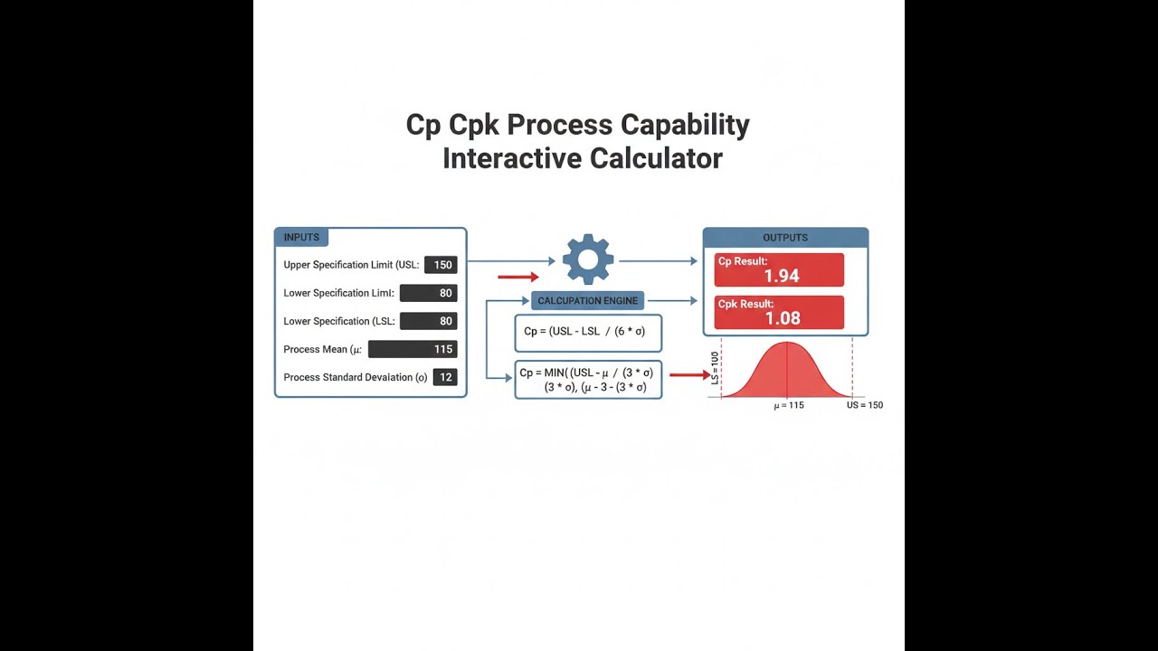
Cp Cpk Process Capability Interactive Calculator
Visualize how process variation fits within specification limits and see real-time capability indices. Adjust process mean and standard deviation to understand the difference between potential (Cp) and actual (Cpk) process capability.
CP (POTENTIAL)
2.00
CPK (ACTUAL)
2.00
SIGMA LEVEL
6.00σ
DEFECT RATE
3 PPM
FIRGELLI Automations — Interactive Engineering Calculators
Formulas & Equations
Use the formula below to calculate process capability (Cp).
Process Capability (Cp)
Cp = (USL - LSL) / (6σ)
Where:
USL = Upper Specification Limit (engineering units)
LSL = Lower Specification Limit (engineering units)
σ = Process standard deviation (short-term, within-subgroup)
6σ = Natural process spread (99.73% of data in normal distribution)
Use the formula below to calculate the process capability index (Cpk).
Process Capability Index (Cpk)
Cpk = min(Cpu, Cpl)
Cpu = (USL - μ) / (3σ)
Cpl = (μ - LSL) / (3σ)
Where:
μ = Process mean (average of measurements)
Cpu = Upper capability index (distance to upper limit)
Cpl = Lower capability index (distance to lower limit)
Cpk always equals the smaller of Cpu and Cpl, representing worst-case capability
Use the formula below to calculate long-term process performance indices (Pp and Ppk).
Process Performance Indices (Pp & Ppk)
Pp = (USL - LSL) / (6σoverall)
Ppk = min[(USL - μ) / (3σoverall), (μ - LSL) / (3σoverall)]
Where:
σoverall = Overall standard deviation (long-term, includes all variation sources)
Pp measures long-term potential performance
Ppk measures long-term actual performance accounting for centering
Use the formula below to calculate the Z-score and estimate defect rate from a Cpk value.
Z-Score and Defect Rate Relationship
Z = Cpk × 3
Where:
Z = Standard score representing distance from mean to nearest specification limit in standard deviations
Approximate PPM (parts per million defects) can be estimated from standard normal distribution tables
6-sigma (Z=6): ~3.4 PPM | 5-sigma (Z=5): ~233 PPM | 4-sigma (Z=4): ~6,210 PPM | 3-sigma (Z=3): ~66,807 PPM
Simple Example
A machined shaft has LSL = 10.00 mm, USL = 10.10 mm, process mean μ = 10.05 mm, and standard deviation σ = 0.010 mm.
- Cp = (10.10 − 10.00) / (6 × 0.010) = 0.10 / 0.060 = 1.67
- Cpu = (10.10 − 10.05) / (3 × 0.010) = 0.05 / 0.030 = 1.67
- Cpl = (10.05 − 10.00) / (3 × 0.010) = 0.05 / 0.030 = 1.67
- Cpk = min(1.67, 1.67) = 1.67 — process is centered and capable
Theory & Engineering Applications
Fundamental Concepts of Process Capability
Process capability analysis forms the statistical foundation for assessing whether a manufacturing process can consistently produce parts within engineering tolerances. Unlike simple pass/fail inspection, capability indices quantify the margin between actual process performance and specification requirements, providing actionable metrics for quality improvement. The distinction between Cp and Cpk reveals a critical insight often missed in introductory treatments: a process can have excellent potential capability (high Cp) while simultaneously failing to meet customer requirements due to poor centering (low Cpk). This dichotomy drives fundamentally different corrective actions — Cp problems require variance reduction through process improvement, while Cpk problems may be solved simply by adjusting the process mean.
The theoretical assumption of normality underlying capability calculations represents both a strength and a practical limitation. While many machining processes produce approximately normal distributions due to the central limit theorem's effect on accumulated random variations, real manufacturing data frequently exhibits skewness, bimodality, or truncation from 100% screening. The conventional 6σ spread encompasses 99.73% of a normal population, but this percentage changes dramatically with distribution shape. A lognormal distribution with coefficient of variation 0.3 — common in chemical processes — may have 95% of data within only 4.2σ rather than 6σ, leading to significant underestimation of defect rates when using standard capability formulas. Advanced practitioners employ Box-Cox transformations or non-parametric capability metrics for non-normal data, but these techniques require substantially larger sample sizes to achieve equivalent statistical confidence.
Short-Term versus Long-Term Capability
The distinction between Cp/Cpk (short-term capability using within-subgroup standard deviation) and Pp/Ppk (long-term performance using overall standard deviation) reveals process behavior across different time scales. Within-subgroup standard deviation captures only the inherent, instantaneous variation of the process — sometimes called "voice of the process" — while filtering out shifts, drifts, and between-subgroup variation. Overall standard deviation includes all sources of variation: tool wear, operator changes, raw material lot differences, environmental fluctuations, and measurement system variability. For stable processes, Pp approximates Cp, but the ratio Cp/Pp provides a powerful diagnostic: values significantly greater than 1.0 indicate the process experiences substantial time-dependent variation that could be reduced through better process control.
In automotive and aerospace applications following AIAG or AS9145 standards, the acceptance criteria typically demand Cpk ≥ 1.33 for critical characteristics and Cpk ≥ 1.67 for safety-critical features. These seemingly arbitrary thresholds encode specific defect rate targets: Cpk = 1.33 corresponds to approximately 63 PPM defect rate (assuming a centered, normal process), while Cpk = 1.67 yields roughly 0.57 PPM — near six-sigma performance. However, the relationship between Cpk and actual defect rate depends critically on the rarely-stated assumption that the process remains centered. A process with inherent Cpk = 1.67 that drifts by 1.5σ from nominal will produce approximately 3.4 PPM defects, the basis of Motorola's original Six Sigma methodology. This 1.5σ shift allowance — controversial among statisticians but pragmatic for industrial application — acknowledges that real processes rarely maintain perfect centering over extended production runs.
Measurement System Impact on Capability Metrics
A frequently overlooked limitation in capability analysis involves measurement system uncertainty. The standard deviation used in Cp and Cpk calculations represents total observed variation, which includes both actual part-to-part variation and measurement system contribution. If measurement repeatability and reproducibility contribute 30% of observed variation (a borderline acceptable measurement system per AIAG guidelines), the calculated capability indices underestimate true process capability by approximately 5%. For precision manufacturing where tolerances approach measurement system resolution — such as bearing journals measured to 0.0001 inch with micrometers having 0.00005 inch resolution — this effect becomes critical. The ratio of tolerance to measurement system uncertainty (called discrimination ratio or "number of distinct categories") should exceed 10:1 to ensure capability calculations reliably reflect process performance rather than measurement limitations.
Worked Example: Precision Shaft Manufacturing
Consider a CNC turning operation producing drive shafts with a diameter specification of 25.000 mm ± 0.040 mm (LSL = 24.960 mm, USL = 25.040 mm). Quality engineers collect 125 measurements over five production shifts using a calibrated coordinate measuring machine with 0.002 mm repeatability. The calculated process mean is μ = 25.018 mm with short-term standard deviation σ = 0.0117 mm (from within-subgroup variation of 25 rational subgroups).
Step 1: Calculate specification parameters
Total tolerance = USL - LSL = 25.040 - 24.960 = 0.080 mm
Specification center = (USL + LSL) / 2 = (25.040 + 24.960) / 2 = 25.000 mm
Process offset from center = |μ - center| = |25.018 - 25.000| = 0.018 mm
Step 2: Calculate process capability (Cp)
Cp = (USL - LSL) / (6σ) = 0.080 / (6 × 0.0117) = 0.080 / 0.0702 = 1.139
This Cp value indicates that if the process were perfectly centered at 25.000 mm, it would be marginally capable (Cp slightly above 1.0), with the natural process spread consuming approximately 88% of the tolerance band.
Step 3: Calculate capability indices accounting for centering
Cpu = (USL - μ) / (3σ) = (25.040 - 25.018) / (3 × 0.0117) = 0.022 / 0.0351 = 0.627
Cpl = (μ - LSL) / (3σ) = (25.018 - 24.960) / (3 × 0.0117) = 0.058 / 0.0351 = 1.652
Cpk = min(Cpu, Cpl) = min(0.627, 1.652) = 0.627
Step 4: Interpret results and estimate defect rate
The dramatic difference between Cp = 1.139 and Cpk = 0.627 immediately indicates a centering problem — the process is shifted significantly toward the upper specification limit. The Cpk value of 0.627 corresponds to approximately Z = 1.88 standard deviations (from Z = Cpk × 3), which translates to roughly 30,000 PPM defect rate on the upper tail using standard normal distribution tables. The asymmetry between Cpu and Cpl confirms the process produces virtually no rejects at the lower limit but significant defects at the upper limit.
Step 5: Calculate required process adjustment
To achieve target Cpk = 1.33, the process must be recentered. The critical distance (minimum distance to either specification limit) should be:
Required distance = Cpk × 3σ = 1.33 × 3 × 0.0117 = 0.0467 mm
Since the tolerance is symmetric and centered at 25.000 mm, optimal centering places the mean at specification center:
Target mean = 25.000 mm
Required adjustment = Current mean - Target mean = 25.018 - 25.000 = -0.018 mm
The CNC program offset should be reduced by 0.018 mm (18 microns). After this adjustment, assuming standard deviation remains constant:
New Cpu = (25.040 - 25.000) / 0.0351 = 1.139
New Cpl = (25.000 - 24.960) / 0.0351 = 1.139
New Cpk = 1.139
This achieves the process's potential capability, reducing estimated defect rate to approximately 1,200 PPM — a 25-fold improvement from simple recentering. To reach Cpk = 1.33, variance reduction would be required, necessitating investigation of tool wear patterns, coolant temperature stability, and workpiece clamping consistency.
Statistical Confidence and Sample Size Requirements
Capability indices calculated from sample data are point estimates subject to sampling uncertainty. The confidence interval width for Cpk depends on both sample size and the true (unknown) capability value, creating a bootstrapping problem in experimental design. For a process with true Cpk = 1.33, a sample of 30 measurements yields 95% confidence interval approximately ±0.24 (ranging from 1.09 to 1.57), while 100 measurements narrows this to ±0.13. AIAG guidelines recommend minimum sample sizes of 100 for initial capability studies and 125 for ongoing monitoring, though these recommendations assume the data represents stable process conditions.
In practice, collecting 25-30 rational subgroups of 4-5 consecutive parts provides better variance estimation than 100 individual measurements, as it separates within-piece from between-piece variation and enables detection of process shifts or trends through control chart analysis performed concurrently with capability assessment.
For additional resources on statistical process control and quality engineering, visit our complete library of engineering calculators, which includes tools for statistical analysis, tolerance stackup, and reliability engineering.
Practical Applications
Scenario: Automotive Supplier Qualification
Jennifer, a quality manager at a Tier 2 automotive supplier, must demonstrate process capability for a new connecting rod machining line before receiving production approval from the OEM customer. The customer specification requires bore diameter of 52.00 mm ± 0.025 mm with mandatory Cpk ≥ 1.67 for this safety-critical dimension. Jennifer collects 150 measurements across 30 subgroups during the production trial, calculating a mean of 52.003 mm and standard deviation of 0.0082 mm. Using the calculator, she determines Cp = 2.03 and Cpk = 1.70, exceeding the customer requirement. However, she notices the process is offset by 3 microns from nominal. By adjusting the CNC program to center the process at exactly 52.000 mm, she improves Cpk to 2.03, matching Cp and providing substantial margin against future process drift. This proactive centering prevents potential quality issues during volume production and demonstrates statistical process control maturity that differentiates her facility during customer audits.
Scenario: Medical Device Continuous Improvement
Dr. Robert Chen, a process engineer at a surgical instrument manufacturer, investigates customer complaints about inconsistent spring force in laparoscopic graspers. The specification calls for 8.0 N ± 1.2 N closing force, but field returns show intermittent weak grip. His initial capability study reveals Cpk = 0.89—well below the medical device industry standard of 1.33—with an estimated 5,700 PPM defect rate. Using the calculator's reverse calculation mode, he determines that achieving Cpk = 1.50 requires reducing process standard deviation from 0.42 N to 0.27 N. Root cause analysis traces excessive variation to inconsistent heat treatment temperature (±8°C variation). After implementing closed-loop PID control reducing temperature variation to ±2°C, the re-qualified process achieves Cpk = 1.58, reducing estimated defect rate to below 50 PPM. The documented capability improvement supports FDA 510(k) submission for the enhanced manufacturing process and eliminates field complaints over the subsequent 18-month monitoring period.
Scenario: Semiconductor Yield Optimization
Maria, a fab process engineer at a semiconductor manufacturer, uses Cp/Cpk analysis to optimize photolithography critical dimension (CD) control for 7nm node production. The design rule specifies CD = 18 nm ± 1.5 nm for gate length, representing an extremely tight tolerance relative to atomic-scale processes. Initial metrology data from 200 die shows mean CD = 18.3 nm with σ = 0.41 nm, yielding Cpk = 0.98—unacceptable for volume production. The calculator reveals that achieving six-sigma capability (Cpk = 2.0) requires reducing σ to 0.25 nm while recentering to 18.0 nm. Maria's team implements advanced process control using feed-forward dose compensation based on upstream film thickness measurements, reducing σ to 0.28 nm. Combined with exposure dose optimization that centers the process, final capability reaches Cpk = 1.79. This improvement increases die yield from 73% to 91%, translating to $2.3 million monthly revenue gain on this single process layer—demonstrating how capability analysis directly links to semiconductor economics where sub-percentage yield improvements justify million-dollar process optimization investments.
Frequently Asked Questions
What is the difference between Cp and Cpk, and which is more important? +
How many samples do I need for a reliable capability study? +
What Cpk value should I target for my process? +
When should I use Pp/Ppk instead of Cp/Cpk? +
Can I calculate capability for non-normal or one-sided specifications? +
What should I do if my Cpk is below the required value? +
Free Engineering Calculators
Explore our complete library of free engineering and physics calculators.
Browse All Calculators →🔗 Explore More Free Engineering Calculators
About the Author
Robbie Dickson — Chief Engineer & Founder, FIRGELLI Automations
Robbie Dickson brings over two decades of engineering expertise to FIRGELLI Automations. With a distinguished career at Rolls-Royce, BMW, and Ford, he has deep expertise in mechanical systems, actuator technology, and precision engineering.
Need to implement these calculations?
Explore the precision-engineered motion control solutions used by top engineers.


