Microscope Resolution Abbe Interactive Calculator

The Abbe diffraction limit defines the fundamental resolution capability of optical microscopes, determining the minimum distance between two point sources that can be distinguished as separate entities. Named after Ernst Abbe who formulated this principle in 1873, this calculator enables precise determination of lateral and axial resolution limits based on wavelength, numerical aperture, and refractive index. Optical engineers, microscopists, and materials scientists rely on these calculations for microscope system design, objective lens selection, and experimental protocol optimization.

📐 Browse all free engineering calculators

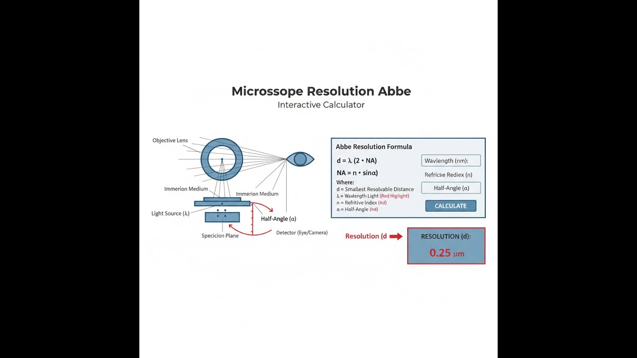
Optical System Diagram

Microscope Resolution Abbe Calculator

Resolution Equations

Theory & Engineering Applications

Fundamental Diffraction Physics and the Abbe Limit

Ernst Abbe's 1873 formulation of optical resolution fundamentally changed microscopy by establishing that the resolution limit stems not from lens imperfections but from the wave nature of light itself. When coherent light passes through a circular aperture, diffraction creates an Airy disk pattern where the central bright region is surrounded by concentric rings of decreasing intensity. The Rayleigh criterion, which uses the 0.61 factor in Abbe's equation, defines resolution as the minimum separation where the central maximum of one Airy disk coincides with the first minimum of the adjacent disk, producing a 26.3% dip in combined intensity between the two points.

The numerical aperture represents the light-gathering power and resolving ability of an objective lens, defined as the product of the refractive index of the imaging medium and the sine of the half-angle of the maximum cone of light entering the lens. This parameter fundamentally constrains resolution because it determines how many diffracted orders from the specimen can be collected. In confocal microscopy and structured illumination systems, engineers exploit the nonlinear relationship between NA and both lateral and axial resolution—note that axial resolution degrades as the square of NA, creating the characteristic elongation of the point spread function along the optical axis.

Immersion Media and High-NA Objectives

The theoretical maximum NA for dry objectives operating in air (n = 1.0) is approximately 0.95, limited by practical lens geometries and working distances. Oil immersion objectives achieve NA values up to 1.6 by replacing the air gap with immersion oil (n ≈ 1.518), closely matching the refractive index of standard cover glass. This eliminates refraction at the glass-air interface, allowing larger cone angles and capturing higher-order diffracted light that would otherwise undergo total internal reflection. Water immersion objectives (NA up to 1.3) serve as a compromise for live-cell imaging where oil can be toxic or impractical.

A critical but often overlooked limitation involves the cover glass thickness specification. Objectives designed for 0.17mm cover glass (#1.5) experience spherical aberration when used with incorrect thickness, degrading both resolution and contrast. The aberration increases dramatically with NA—a 1.4 NA objective shows significant degradation with just 10 micrometers of deviation from nominal thickness, while a 0.5 NA objective tolerates much larger errors. Modern correction collars on high-NA objectives compensate for this by adjusting internal lens spacing.

Wavelength Selection and Multi-Color Imaging

The linear dependence of resolution on wavelength creates a direct trade-off between resolution and fluorophore selection in fluorescence microscopy. Violet lasers at 405nm provide 26.5% better lateral resolution than red lasers at 640nm when using identical NA objectives. However, shorter wavelengths increase phototoxicity in live cells and often provide poorer penetration depth in thick specimens due to increased scattering. This drives sophisticated microscope designs using sequential imaging with multiple wavelengths, where registration algorithms must account for chromatic aberration and the wavelength-dependent point spread function.

In confocal systems, the effective resolution improves approximately by the square root of two compared to widefield microscopy due to the multiplicative effect of excitation and emission point spread functions. This relationship means a 488nm confocal system achieves resolution comparable to a 345nm widefield system—a wavelength not practical for most applications due to UV absorption by optical materials and severe cellular damage.

Axial Resolution and Three-Dimensional Imaging

The axial resolution equation reveals that depth discrimination is fundamentally worse than lateral resolution, typically by a factor of 2-3 for high-NA objectives. This anisotropic resolution creates elongated point spread functions that complicate three-dimensional reconstruction and quantitative volume measurements. Deconvolution algorithms can partially compensate by using knowledge of the theoretical point spread function to reassign out-of-focus light, but these techniques require careful calibration and fail when noise levels become significant.

The squared dependence of axial resolution on NA means that improvements in NA provide dramatically better depth discrimination—increasing NA from 1.3 to 1.4 improves axial resolution by 16.5%. This nonlinear relationship explains why manufacturers invest heavily in developing ultra-high NA objectives despite the engineering challenges of maintaining field flatness, working distance, and chromatic correction at these extreme parameters.

Worked Engineering Example: Confocal Microscope Design

Problem: A biomedical research laboratory is designing a confocal fluorescence microscope for imaging subcellular structures in fixed tissue sections. The primary fluorophore emits at 520nm (green). The team must determine whether a 1.3 NA water immersion objective or a 1.4 NA oil immersion objective is required to resolve structures with 180nm lateral spacing. Additionally, they need to calculate the axial resolution and determine the optimal pinhole size for the confocal aperture.

Given Data:

• Emission wavelength: λ = 520 nm
• Target lateral resolution: d_target = 180 nm
• Option A: NA = 1.3 (water immersion, n = 1.33)
• Option B: NA = 1.4 (oil immersion, n = 1.518)
• Confocal improvement factor: √2 ≈ 1.414

Solution - Part 1: Lateral Resolution Calculation

For widefield microscopy using Option A (NA = 1.3):

d_A = 0.61λ / NA = (0.61 × 520 nm) / 1.3 = 317.2 nm / 1.3 = 244.0 nm

For confocal microscopy with Option A:

d_confocal,A = 244.0 nm / 1.414 = 172.5 nm

For widefield microscopy using Option B (NA = 1.4):

d_B = (0.61 × 520 nm) / 1.4 = 317.2 nm / 1.4 = 226.6 nm

For confocal microscopy with Option B:

d_confocal,B = 226.6 nm / 1.414 = 160.3 nm

Analysis: The 1.3 NA water immersion objective achieves 172.5 nm confocal resolution, which meets the 180 nm requirement with a 4% margin. The 1.4 NA oil objective provides 160.3 nm resolution, exceeding requirements by 11%.

Solution - Part 2: Axial Resolution Calculation

For Option A (water immersion):

z_A = 2nλ / NA² = (2 × 1.33 × 520 nm) / (1.3²) = 1383.2 nm / 1.69 = 818.5 nm

For confocal mode:

z_confocal,A = 818.5 nm / 1.414 = 578.9 nm

For Option B (oil immersion):

z_B = (2 × 1.518 × 520 nm) / (1.4²) = 1578.7 nm / 1.96 = 805.5 nm

For confocal mode:

z_confocal,B = 805.5 nm / 1.414 = 569.7 nm

Solution - Part 3: Optimal Pinhole Diameter

The optimal confocal pinhole diameter equals 1.0 Airy unit, which corresponds to the diameter of the first Airy disk minimum in the detection path. For Option B (oil, NA = 1.4), assuming a 200mm tube lens focal length and 520nm emission:

Airy disk diameter = 1.22λf / (NA × M_obj) where M_obj is objective magnification (assume 63x):

Airy diameter = (1.22 × 520 nm × 200 mm) / (1.4 × 63) = 127,440 nm·mm / 88.2 = 1445 μm ≈ 31.7 μm at the pinhole plane

Recommendation: Select the 1.4 NA oil immersion objective. While the 1.3 NA water objective technically meets requirements, the oil objective provides superior axial resolution (569.7 nm vs 578.9 nm) and greater margin in lateral resolution. The oil interface also eliminates spherical aberration from refractive index mismatch with the cover glass. Use a pinhole diameter of 30-35 μm (approximately 1.0 Airy units) for optimal optical sectioning while maintaining adequate signal levels.

Beyond the Diffraction Limit: Super-Resolution Techniques

Modern super-resolution microscopy methods circumvent the Abbe limit through various mechanisms. Stimulated emission depletion (STED) microscopy uses a donut-shaped depletion beam to suppress fluorescence everywhere except a sub-diffraction region, effectively shrinking the point spread function. Structured illumination microscopy (SIM) uses patterned illumination to encode high-spatial-frequency information into the passband of the optical system, achieving approximately 2x resolution improvement. Single-molecule localization methods like PALM and STORM achieve 20-30nm resolution by sequentially imaging and precisely localizing individual fluorophores, though at the cost of temporal resolution.

These techniques trade various parameters—acquisition speed, photobleaching, complexity, or applicability to live samples—for improved resolution. Understanding the Abbe limit remains critical even in super-resolution work because it defines the starting point from which these advanced methods build their improvements and constrains fundamental parameters like the photon budget available for localization precision.

Practical Applications

Frequently Asked Questions