Knowing how fast a shear wave travels through a material tells you almost everything about that material's mechanical character — its stiffness, its phase state, and how it will behave under dynamic loading. Use this Shear Wave Velocity Calculator to calculate shear wave velocity, shear modulus, density, wavelength, or frequency using elastic constants and material density. That matters across seismology, non-destructive testing of welds and pressure vessels, and geotechnical site classification for earthquake engineering. This page covers the core formulas, a worked steel inspection example, plain-English theory, and a full FAQ.
What is Shear Wave Velocity?
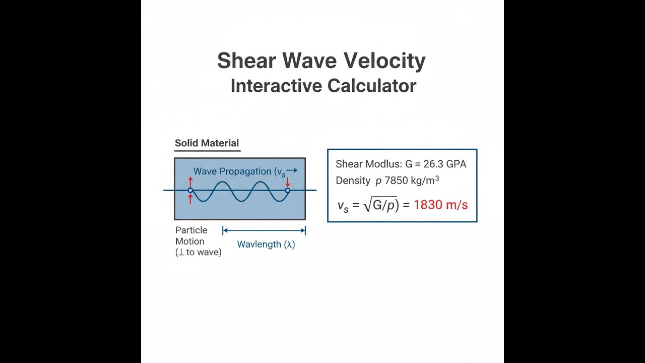
Shear wave velocity is the speed at which a transverse elastic wave — one where the material moves side-to-side rather than back-and-forth — travels through a solid. It depends on how stiff the material is in shear and how dense it is. Stiffer materials carry shear waves faster. Denser materials slow them down.
Simple Explanation
Think of a shear wave like a ripple traveling along a stretched rubber band when you flick it sideways — the band moves up and down while the wave travels along its length. In a solid material, the same thing happens at a microscopic scale: layers of atoms displace sideways as the wave passes through. The stiffer the material resists that sideways push, the faster the wave travels — and crucially, fluids like water or air have zero resistance to sideways push, so shear waves simply cannot exist in them.
📐 Browse all 1000+ Interactive Calculators
Shear Wave Propagation Diagram

Shear Wave Velocity Calculator
How to Use This Calculator
- Select your calculation mode from the dropdown — choose what you want to solve for (velocity, shear modulus, density, wavelength, or frequency).
- Enter the required input values in the fields that appear — units are shown below each input field.
- Check your values are positive and physically reasonable before proceeding.
- Click Calculate to see your result.
Shear Wave Velocity Interactive Visualizer
Watch how shear waves propagate through materials with different stiffness and density properties. Adjust material parameters to see real-time effects on wave velocity and transmission characteristics.
VELOCITY
3200 m/s
WAVELENGTH
6.4 m
IMPEDANCE
25.0 MRayl
FIRGELLI Automations — Interactive Engineering Calculators
Shear Wave Velocity Equations
Use the formula below to calculate shear wave velocity from shear modulus and density.
vs = √(G/ρ)
where:
- vs = shear wave velocity (m/s)
- G = shear modulus or modulus of rigidity (Pa or N/m²)
- ρ = material density (kg/m³)
Use the formula below to calculate shear modulus from Young's modulus and Poisson's ratio.
G = E / [2(1 + ν)]
where:
- E = Young's modulus (Pa)
- ν = Poisson's ratio (dimensionless)
Use the formula below to calculate wavelength from shear wave velocity and frequency.
λ = vs / f
where:
- λ = wavelength (m)
- f = frequency (Hz)
Use the formula below to calculate shear acoustic impedance.
Zs = ρ × vs
where:
- Zs = shear acoustic impedance (Rayl or kg/(m²·s))
Simple Example
A soil sample has a shear modulus G = 50 MPa (0.05 GPa) and a density ρ = 2000 kg/m³.
vs = √(G/ρ) = √(50,000,000 / 2000) = √25,000 = 158.1 m/s
That velocity classifies the soil as soft ground — well below the 180 m/s threshold used in seismic site classification codes.
Theory & Practical Applications
Fundamental Physics of Shear Wave Propagation
Shear waves propagate through solid materials via transverse particle displacement, where material elements oscillate perpendicular to the direction of wave travel. This distinguishes them fundamentally from longitudinal (compressional) waves where particle motion parallels propagation. The physical mechanism involves shear stress and strain: when one layer of material is displaced laterally relative to an adjacent layer, elastic restoring forces arise that are proportional to the shear modulus. The velocity of propagation depends on the material's resistance to shear deformation (shear modulus G) and its inertial resistance to acceleration (density ρ).
A critical but often overlooked aspect is that shear wave velocity is ALWAYS lower than compressional wave velocity in the same material. For most engineering materials, the ratio vs/vp ranges from 0.5 to 0.7. This velocity difference is the fundamental principle behind seismic wave arrival time analysis—P-waves arrive first, followed by S-waves, and the time separation reveals distance to the source. In ultrasonic testing, this velocity differential affects inspection techniques: shear wave transducers must operate at different frequencies than longitudinal transducers to achieve equivalent wavelengths and resolution.
Material Property Relationships and Elastic Constant Determination
The shear modulus G represents a material's resistance to shape change under shear stress while maintaining constant volume. For isotropic materials, three of the four elastic constants (Young's modulus E, shear modulus G, bulk modulus K, Poisson's ratio ν) uniquely determine the fourth. The relationship G = E/[2(1+ν)] enables shear wave velocity measurements to extract Poisson's ratio when combined with longitudinal wave data. This dual-wave approach is standard in geophysical characterization and advanced materials testing.
Temperature dependence introduces significant practical complications. Shear modulus typically decreases with increasing temperature due to reduced interatomic bonding strength, while density changes are comparatively minor. For steel between 20°C and 200°C, shear wave velocity can decrease by 8-12%, creating measurement errors if not properly corrected. In high-temperature industrial monitoring applications—such as pipeline integrity assessment or turbine blade inspection—temperature-compensated velocity tables become essential calibration references.
Seismology and Geotechnical Engineering Applications
In earthquake seismology, shear wave velocity profiles of subsurface soil and rock layers determine site amplification characteristics during ground shaking. The Vs30 parameter—average shear wave velocity in the top 30 meters—is the primary metric for seismic site classification in building codes worldwide. Sites with Vs30 below 180 m/s (soft clays) experience dramatic amplification of earthquake motions, while rock sites exceeding 760 m/s show minimal amplification. This classification directly influences design ground motion specifications and construction requirements.
Crosshole seismic testing and surface wave methods (MASW, SASW) measure in-situ shear wave velocities for foundation design and liquefaction assessment. A critical engineering insight: loose saturated sands with Vs below approximately 200 m/s are highly susceptible to liquefaction—a catastrophic loss of strength during cyclic loading where soil behaves temporarily as a viscous liquid. This threshold isn't arbitrary; it corresponds to relative density ranges where particle rearrangement under cyclic stress can rapidly increase pore pressures beyond confining stress.
Non-Destructive Testing and Materials Characterization
Ultrasonic shear wave testing operates typically between 500 kHz and 10 MHz for flaw detection in metals, composites, and ceramics. At 2.25 MHz in steel (vs ≈ 3240 m/s), the wavelength is 1.44 mm, providing resolution sufficient to detect sub-millimeter cracks and inclusions. Angle beam transducers generate shear waves via mode conversion at interfaces, with wedge angles calculated using Snell's law to achieve desired refraction angles—typically 45°, 60°, or 70° for weld inspection.
A subtle but crucial limitation: shear wave attenuation increases dramatically with frequency and grain size. In coarse-grained cast materials or austenitic stainless steel welds, scattering attenuation can render shear wave inspection impractical above 2 MHz, forcing reliance on lower-frequency longitudinal waves with reduced resolution. The transition from specular reflection (flaw dimension much larger than wavelength) to Rayleigh scattering (flaw dimension comparable to wavelength) occurs around D/λ = 1, fundamentally limiting defect sizing accuracy.
Advanced Applications in Material Science
Laser ultrasonic systems measure shear wave velocity in extreme environments—temperatures exceeding 1500°C, vacuum conditions, or highly radioactive zones—where conventional transducers fail. Pulsed laser ablation generates broadband elastic waves, while interferometric detection measures surface displacements with picometer resolution. This enables real-time monitoring of phase transformations, precipitation hardening, and microstructural evolution where elastic properties change continuously.
Resonant ultrasound spectroscopy (RUS) determines the complete elastic constant tensor from resonant frequency measurements, requiring shear wave velocity data for validation. For anisotropic materials like fiber composites or single crystals, up to 21 independent elastic constants may exist, and shear wave velocity varies with propagation and polarization directions. Aerospace composite qualification relies on these measurements to verify fiber orientation, resin cure state, and damage accumulation through elastic property changes.
Worked Example: Steel Plate Inspection Design
An engineer must design an ultrasonic shear wave inspection system for detecting transverse cracks in a 50 mm thick ASTM A36 structural steel plate used in a pressure vessel. Available transducers operate at 2.25 MHz and 5.0 MHz. The steel has Young's modulus E = 200 GPa, Poisson's ratio ν = 0.30, and density ρ = 7850 kg/m³. Specification requires detecting cracks with minimum dimension 3 mm perpendicular to the wave path.
Step 1: Calculate shear modulus from elastic constants
Using the relationship between Young's modulus and shear modulus:
G = E / [2(1 + ν)] = 200 GPa / [2(1 + 0.30)] = 200 / 2.60 = 76.92 GPa
Converting to standard SI units: G = 76.92 × 10°— Pa
Step 2: Calculate shear wave velocity
vs = √(G/ρ) = √(76.92 × 10⁹ / 7850) = √(9.798 × 10°) = 3130 m/s
Step 3: Calculate wavelength for each transducer frequency
For 2.25 MHz: λ = vs/f = 3130 / (2.25 × 10⁶) = 0.001391 m = 1.391 mm
For 5.0 MHz: λ = vs/f = 3130 / (5.0 × 10⁶) = 0.000626 m = 0.626 mm
Step 4: Evaluate detection capability using wavelength criterion
The standard detection criterion requires flaw dimension D ≥ λ/2 for reliable detection (Rayleigh scattering regime begins near D ≈ λ). For the required 3 mm minimum crack:
2.25 MHz: D/λ = 3.0 / 1.391 = 2.16 (acceptable, well into geometric reflection regime)
5.0 MHz: D/λ = 3.0 / 0.626 = 4.79 (excellent sensitivity, higher resolution)
Step 5: Calculate beam spread and near-field distance
For a 12 mm diameter transducer at 5.0 MHz:
Near-field length N = D²f / (4vs) = (0.012)² × (5.0 × 10⁶) / (4 × 3130) = 45.8 mm
Since plate thickness (50 mm) slightly exceeds near-field length, inspection occurs in the transition zone—acceptable but not optimal. A 2.25 MHz transducer would have N = 20.6 mm, placing the far surface well into the far field with more predictable beam characteristics.
Step 6: Calculate acoustic impedance for interface analysis
Zs = ρ × vs = 7850 × 3130 = 24.57 × 10⁶ Rayl = 24.57 MRayl
This impedance determines coupling efficiency and reflection coefficients at the transducer-steel interface, affecting calibration requirements.
Conclusion: The 2.25 MHz transducer provides adequate resolution (λ = 1.391 mm) for detecting 3 mm cracks while ensuring far-field inspection conditions throughout the plate thickness. The 5.0 MHz option offers superior resolution but operates partially in the near field, complicating beam modeling and potentially creating dead zones. Material attenuation measurements would provide the final selection criterion—if grain scattering is significant, the lower frequency becomes essential despite reduced resolution. This example demonstrates why shear wave velocity calculation is the critical first step in ultrasonic inspection system design.
Coupling to Broader Engineering Calculations
Shear wave velocity connects to multiple engineering analysis domains. In vibration analysis, shear deformation in beams and plates contributes to dynamic response at wavelengths approaching structural dimensions—the Timoshenko beam theory correction becomes significant when wavelength λ ≈ 10h (where h is thickness), requiring accurate shear modulus values derived from velocity measurements. For composite materials, the through-thickness shear wave velocity directly relates to interlaminar shear strength, a critical failure mode parameter.
For those investigating related wave phenomena, the engineering calculator library provides additional resources on compressional wave velocity, acoustic impedance calculations, and Rayleigh surface wave propagation—all interconnected through the elastic properties accessed via shear wave measurements.
Frequently Asked Questions
Free Engineering Calculators
Explore our complete library of free engineering and physics calculators.
Browse All Calculators →🔗 Explore More Free Engineering Calculators
About the Author
Robbie Dickson — Chief Engineer & Founder, FIRGELLI Automations
Robbie Dickson brings over two decades of engineering expertise to FIRGELLI Automations. With a distinguished career at Rolls-Royce, BMW, and Ford, he has deep expertise in mechanical systems, actuator technology, and precision engineering.
Need to implement these calculations?
Explore the precision-engineered motion control solutions used by top engineers.


