Shear Wave Velocity Interactive Calculator

If you know the speed of a shear wave in a material, you can quickly estimate its stiffness, whether it’s solid, and get a handle on how it will respond to shock or vibration. The calculator below lets you work out shear wave velocity, modulus, density, wavelength, or frequency based on the core elastic constants. This kind of calculation comes up in seismology, weld inspections, and soil tests for earthquake design. What follows are the main formulas, a worked example with steel, practical theory, and a focused FAQ.

What is Shear Wave Velocity?

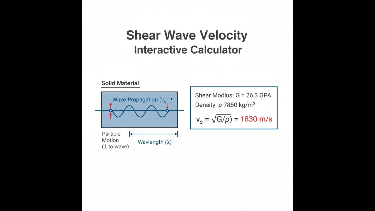
Shear wave velocity is how fast a transverse wave moves through a solid—the kind of wave where particles shift side-to-side as the wave passes, rather than moving in the same direction as the wave itself. Materials with higher shear stiffness send these waves faster. Denser materials slow them down. So, the stiffer and lighter the solid, the faster a shear wave travels through it.

Simple Explanation

If you flick a stretched rubber band sideways, the ripple you see is a shear wave: the band goes up and down, but the wave itself moves along the length. In solids, the same thing is happening but at the atomic level—layers of atoms slip sideways a tiny bit as the wave goes by. If a material barely resists this sideways motion, the wave crawls through; if it resists strongly, the wave zips along. Liquids and gases don’t resist this kind of movement at all, so shear waves just don’t happen in them.

📐 Browse all 1000+ Interactive Calculators

Shear Wave Propagation Diagram

Shear Wave Velocity Calculator

How to Use This Calculator

1. Select your calculation mode from the dropdown — choose what you want to solve for (velocity, shear modulus, density, wavelength, or frequency).
2. Enter the required input values in the fields that appear — units are shown below each input field.
3. Check your values are positive and physically reasonable before proceeding.
4. Click Calculate to see your result.

Shear Wave Velocity Equations

The formula below gives you the shear wave speed if you know shear modulus and density.

To get shear modulus from Young's modulus and Poisson’s ratio, use this:

Wavelength comes out of wave speed divided by frequency:

For acoustic impedance (used in wave reflections and coupling):

Simple Example

Say a soil sample’s shear modulus is 50 MPa (0.05 GPa), and density is 2000 kg/m³.

v_s = √(G/ρ) = √(50,000,000 / 2000) = √25,000 = 158.1 m/s

You’d consider this soft ground—well under the 180 m/s cutoff often used in seismic code classifications.

Theory & Practical Applications

Fundamental Physics of Shear Wave Propagation

Shear waves push particles sideways, perpendicular to the wave direction. That’s different from compressional (P) waves, where particles move in the same direction as the wave. What matters most is how hard it is to shear the material (shear modulus G), and how much mass you’re moving (density ρ). That’s why the formula is as simple as v_s = √(G/ρ).

Important to remember: shear waves are always slower than compressional waves in the same stuff. The typical ratio in engineering materials is v_s/v_p = 0.5 … 0.7. Seismologists use this time gap (P-waves first, S-waves second) to figure out distances to earthquakes, and in ultrasonic testing, you need to consider that your equipment has to be set up differently for each wave type to get similar inspection detail—the required frequencies don’t match up.

Material Property Relationships and Elastic Constant Determination

The shear modulus tells you how much a material resists changing shape at fixed volume. For most metals and isotropic solids, if you have any three of Young’s modulus, shear modulus, bulk modulus, and Poisson’s ratio, the last one is fixed. G = E / [2(1+ν)] is the usual route, and by measuring both shear and longitudinal wave speeds, you can back out Poisson’s ratio. This is how labs get a full elastic profile for new materials or do in-situ checks on rock or soil for geotech.

Temperature messes with results. As temperature goes up, shear modulus drops more than density changes. In something like steel, you can lose 8–12% of shear wave speed between room temperature and 200°C. For any high-temperature industrial monitoring (like turbines), you really need to know how wave speed shifts with temperature or you’ll get the wrong material properties from your readings.

Seismology and Geotechnical Engineering Applications

For earthquake engineering, the key input is how fast a shear wave travels through the first 30 m of site geology—this is the Vs₃₀ value. Sites with Vs₃₀ below 180 m/s (usually soft clay or peat) can experience major amplification of earthquake shaking. Rock sites with Vs₃₀ above 760 m/s have much lower amplification. This Stiffness number goes directly into seismic building codes and dictates construction details.

To actually measure Vs in the ground, crosshole and surface wave methods are typical. There’s a practical cutoff: loose, saturated sand below about 200 m/s for Vs is likely to liquefy in an earthquake—it loses all strength temporarily. This isn’t just a rule of thumb; it matches bulk geotechnical test data showing rapid strength loss at low Vs values.

Non-Destructive Testing and Materials Characterization

In the lab or field, ultrasonic shear wave testing for metals typically runs between 500 kHz and 10 MHz. Take steel for instance: at 2.25 MHz and vs ≈ 3240 m/s, your wavelength is 1.44 mm. That’s fine enough to see sub-millimeter flaws. With weld inspection, probe wedges are cut for specific angles (usually 45°, 60°, or 70°) to deliberately make a shear wave, using Snell’s law. Getting the angle wrong means you won’t even “see” the weld zone properly.

One catch: the higher the frequency (and the bigger the grain size), the more your wave gets scattered and attenuated. In cast steel or stainless welds, above 2 MHz, you can lose so much signal to scattering that you can’t find small cracks. Flaw detection is best when the crack is at least about half a wavelength or more—the math flips around D/λ ≈ 1. Once you get into the same size as the wavelength, precision goes down fast.

Advanced Applications in Material Science

In some environments—like temperatures over 1500°C, strong radiation, or hard-to-reach parts—classic transducers don’t work. Here, you use laser ultrasonics: firing a pulse at the surface to create elastic waves, and then picking them up with sensitive detectors. This method lets you watch property changes in real time, for example during heat treating or solid-state phase change, where stiffness can change as the structure does.

Resonant ultrasound spectroscopy (RUS) is used to map out the full set of elastic constants for complex materials such as fiber composites and single crystals. These materials can have shear velocity that varies depending on direction—fiber direction, for instance, in aerospace composites. You need wave measurements along multiple axes to catch this and qualify the part.

Worked Example: Steel Plate Inspection Design

Let’s say you need to design an ultrasonic system to catch transverse cracks in a 50 mm thick ASTM A36 steel plate (e.g. a pressure vessel). You’ve got two probes: one at 2.25 MHz, one at 5.0 MHz. Material stats: E = 200 GPa, ν = 0.30, ρ = 7850 kg/m³. You’re told to spot cracks down to 3 mm across.

Step 1: Calculate shear modulus from elastic constants

G = E / [2(1 + ν)] = 200 GPa / [2(1 + 0.30)] = 200 / 2.60 = 76.92 GPa

Which is G = 76.92 × 10⁹ Pa.

Step 2: Calculate shear wave velocity

v_s = √(G/ρ) = √(76.92 × 10⁹ / 7850) = √(9.798 × 10⁶) = 3130 m/s

Step 3: Calculate wavelength for each transducer frequency

For 2.25 MHz: λ = 3130 / (2.25 × 10⁶) = 0.001391 m = 1.391 mm

For 5.0 MHz: λ = 3130 / (5.0 × 10⁶) = 0.000626 m = 0.626 mm

Step 4: Check detection limit using wavelength

The practical limit: flaw size D ≥ λ/2. For a 3 mm crack:

2.25 MHz: D/λ = 3.0 / 1.391 = 2.16 (in geometric/reflective regime, detection is reliable)

5.0 MHz: D/λ = 3.0 / 0.626 = 4.79 (even better resolution, but more susceptible to attenuation)

Step 5: Look at beam spread and near-field distance

For a 12 mm diameter probe at 5.0 MHz:

Near-field N = D²f / (4v_s) = (0.012)² × (5.0 × 10⁶) / (4 × 3130) = 45.8 mm

The plate is just thicker than this (50 mm), so the inspection spot is at the edge of the near field. With the 2.25 MHz probe, near field is about 20.6 mm, giving a more uniform beam in the relevant part of the plate.

Step 6: Work out acoustic impedance

Z_s = 7850 × 3130 = 24.57 × 10⁶ Rayl = 24.57 MRayl

This number affects how well your probe couples to the steel and how much signal you lose at the interface—matters for calibration.

Conclusion: The 2.25 MHz probe gives enough resolution to pick up 3 mm cracks, and you’re safely in the far field for most of the plate. The 5.0 MHz unit gives better theoretical resolution but can be affected by scatter and dead zones. Real-world experience says: pick the lower frequency if you want reliability in thick or coarse-grained material, unless lab tests prove the higher frequency works for your case. Always start by calculating wave velocity; it sets up everything else in ultrasonic NDT design.

Coupling to Broader Engineering Calculations

Shear wave velocity comes up far beyond NDT or geotech. For vibration problems in beams and plates, especially at high frequencies or with thick sections, shear deformation alters the resonance modes—Timoshenko beam theory needs a proper G value, which you can only get from wave speed or direct modulus data. With composites, through-thickness shear wave velocity is a direct indicator for interlaminar shear strength: if those numbers are off, you may have a weak bond between laminate layers.

If you’re working on anything involving wave propagation, it’s worth checking related calculations: compressional waves, impedance matching, and surface (Rayleigh) waves—all use these same base properties. The engineering calculator library has tools for those as well.

Frequently Asked Questions