Estimating how fast water moves through soil is something you deal with right at the start of most earthworks, drainage, and groundwater projects. You can’t really size a pump or pick your drainage aggregate until you have a realistic permeability value. This calculator lets you work out hydraulic conductivity (permeability) from grain size—using the main empirical formulas like Hazen, Kozeny-Carman, Breyer, Slichter, and Terzaghi. It’s useful anywhere water flow depends on granular soil—foundation dewatering, aquifer assessment, drainage blanket design, or predicting how a contaminant travels. Below, you’ll find the actual math, a worked example, background notes, and a FAQ.
What is soil permeability from grain size?
Soil permeability, or hydraulic conductivity, tells you how readily water moves through a soil. Grain size calculators estimate permeability from particle size data—mainly by looking at the effective grain diameter—so you can get a quick answer without running a full permeability test in the lab.
Simple Explanation
Imagine you have a bucket of marbles. If the marbles are big, water runs through fast because the gaps between them are large. If the “grains” are smaller and pack tighter, the gaps for water to move shrink, so flow slows down. These grain size calculators use that logic—bigger grains, higher permeability—to give you a first-pass estimate you can use before running more detailed tests.
📐 Browse all 1000+ Interactive Calculators
Diagram

How to Use This Calculator
- Select your calculation method from the Calculation Mode dropdown — Hazen, Kozeny-Carman, Breyer, Slichter, Terzaghi, or Reverse.
- Enter your effective grain size D₁₀ in millimetres (and porosity or void ratio if your chosen method requires them).
- Enter the field water temperature in °C so the calculator can apply the viscosity correction.
- Click Calculate to see your result.
Permeability Grain Size Calculator
This calculator is intended for education, concept evaluation, and preliminary design. Results are based on the equations and assumptions described on this page, but cannot account for every real-world load case, tolerance, material property, environmental condition, installation detail, safety factor, code, or regulatory requirement. Verify all inputs, assumptions, units, and results independently before selecting components or using the result in a real application. Safety-critical, structural, medical, lifting, transportation, or regulated applications must be reviewed by a qualified engineer.
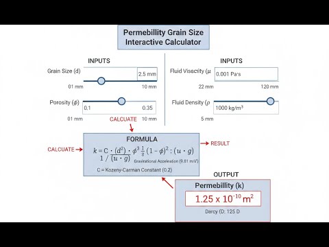
Permeability Grain Size Interactive Visualizer
This visual shows how changing grain size alters water flow. You can adjust parameters and immediately see the effect on permeability using several common empirical formulas. It’s a fast way to get a sense for just how sensitive drainage is to even small grain size changes.
HAZEN k (cm/s)
2.3×10⁻³
KOZENY-CARMAN
1.8×10⁻³
CLASSIFICATION
MED SAND
FIRGELLI Automations — Interactive Engineering Calculators
Equations & Variables
The Hazen equation below is simple and often gets you close if the sand is uniform and clean.
Hazen Equation (1892)
k = C · D₁₀²
Where:
- k = hydraulic conductivity (permeability) at 20°C (cm/s)
- C = Hazen coefficient (typically 1.0 for cm/s when D₁₀ in cm, or 0.01 when D₁₀ in mm)
- D₁₀ = effective grain size, 10% passing diameter (mm)
Valid for uniformly graded fine to medium sands with D₁₀ between 0.1 and 3.0 mm and uniformity coefficient Cu less than 5.
For materials that aren’t so uniform or when you know porosity, the Kozeny-Carman equation will handle more situations, but needs more data.
Kozeny-Carman Equation
k = (D₁₀² · n³) / (180 · (1 - n)²)
Where:
- k = hydraulic conductivity (cm/s)
- D₁₀ = effective grain size (cm)
- n = porosity (dimensionless, 0 to 1)
Theoretical derivation based on flow through idealized porous media; applicable across wider range of soil types when porosity is known.
The Breyer equation is also widely used. It’s most applicable when you’re in that intermediate ground—neither clean uniform sand nor full of fines.
Breyer Equation
k = 0.0060 · D₁₀²
Where:
- k = hydraulic conductivity (cm/s)
- D₁₀ = effective grain size (cm)
- 0.0060 = empirical Breyer coefficient
Hydraulic conductivity depends on water temperature because viscosity changes. If you want your answer to match what happens on site, use the temperature correction formula below.
Temperature Correction
kT = k₂₀ · (μ₂₀ / μT)
Where:
- kT = permeability at field temperature T (cm/s)
- k₂₀ = permeability at standard 20°C (cm/s)
- μ₂₀ = dynamic viscosity of water at 20°C
- μT = dynamic viscosity at temperature T
Simplified empirical approximation: viscosity ratio → (1 + 0.0337T + 0.000221T²) / (1 + 0.0337·20 + 0.000221·20²)
Simple Example
Using the Hazen equation for a clean medium sand:
- D₁₀ = 0.3 mm, temperature = 20°C
- k₂₀ = 0.01 × (0.3)² = 0.01 × 0.09 = 0.0009 cm/s
- Uniformity coefficient Cu = 2.8 — within Hazen's valid range
- Result: k₂₀ = 9.0 × 10⁻⁴ cm/s — classified as fine sand with good drainage
Theory & Engineering Applications
Fundamental Relationship Between Grain Size and Permeability
Water mainly flows through the spaces—or voids—between grains. The best way to estimate how open these paths are is by looking at grain size distribution. The D₁₀ value is often used because it represents the size where only 10% of the sample is finer. Hazen’s work (from sand filters, late 1800s US water treatment) showed that permeability scales pretty closely with the square of D₁₀ for clean, uniform sands. The physics foundation is that both the total area for flow and the hydraulic radius go up as grains get bigger, so flow goes up with roughly D₁₀ squared. That’s where the simple Hazen k ∝ D₁₀² comes from.
D₁₀ is handy because it focuses on the size of pores that really limit flow—the smallest passages between grains. Hazen's original numbers were from cold filter sand, but nowadays we use values standardized at 20°C and apply corrections for temperature, since water gets less viscous as it warms.
Limitations and Non-Obvious Considerations
Grain-size formulas like Hazen are quick, but you have to know when not to trust them. If the soil isn’t uniform—say, a wide range of grain sizes (Cu > 5)—the formula may overestimate by a wide margin. That’s because finer particles block larger voids, and the natural mix can choke off flow: just having a big D₁₀ isn’t enough if 15% of your sample is fines. The prediction will give you a number, but in practice, actual permeability could be 5 or 10 times less than calculated. Always check for the presence of fines—just a bit of silt or clay can easily halve calculated permeability. Lab test results on disturbed samples will often look far better than what actually happens in the ground.
Another limitation: soil structure (the way the grains are arranged) changes things. Horizontal layering, for example, almost always means horizontal permeability will be higher than vertical (sometimes by a factor of 2–5). Compaction isn’t just a density issue: the way you compact the soil changes the flow path geometry. Vibro-compacted sand can drain better than the same sand compacted by rolling or squeezing—sometimes 40% higher, even if D₁₀ is identical.
Engineering Applications Across Multiple Disciplines
Most engineers use grain-size-to-permeability methods for early design work: if you’re logging a site and have sieve data from drilling, these equations let you do rough sizing of pumps, drainage blankets, or wet well discharge rates while waiting for full permeability tests. For example, if you need to decide if excavation dewatering will require big wellpoints or just a sump, quick D₁₀ estimates help you. If your sand has k = 0.08 cm/s, you’ll need much more aggressive pumping than with k = 0.003 cm/s. Environmental consultants use these calculations to budget how hard it will be to clean up a spill or how fast a plume will spread in groundwater: the numbers guide how many wells you’ll need and whether your plan is even feasible before committing to expensive pilot studies. Pavement designers use grain size as a check to select base layers for drainage. Highway specs often require a minimum k calculated from D₁₀ to avoid frost damage or water-logging below the pavement, even at the design phase.
In environmental and hydrogeology work, grain size values help estimate aquifer properties for initial models—plume velocity, time to flush a contaminant, or spacing of recovery wells. Layered soils with different D₁₀ values split flow unevenly; most water will go through the cleanest, coarsest sand, even if it’s not the thickest layer. Not considering this can send modeling way off track.
For pavement and infrastructure, specs may give you a minimum D₁₀ (for example, D₁₀ ≥ 0.6 mm for open-graded layers to hit a certain drainage rate). If you substitute a marginal or finer material for cost, drainage falls off fast—sometimes failing serviceability requirements after a wet season. These equations help you make that cutoff call up front without waiting months for special-order materials.
Worked Example: Dewatering Design for Foundation Excavation
Suppose you’re working on a downtown project that involves digging below the water table—foundation to 4.2 m, water encountered at 2.8 m. Sandy layer sieve results: D₁₀ = 0.31 mm, D₆₀ = 0.89 mm, so Cu = 0.89/0.31 = ~2.9 (well within Hazen’s valid range). Groundwater at 14°C.
Step 1: Calculate uniformity coefficient
Cu = D₆₀ / D₁₀ = 0.89 mm / 0.31 mm = 2.87
Since Cu is less than 5, Hazen equation is applicable.
Step 2: Apply Hazen equation for k at 20°C
k₂₀ = 0.01 × D₁₀² = 0.01 × (0.31)² = 0.01 × 0.0961 = 0.000961 cm/s
Step 3: Apply temperature correction for field conditions at 14°C
Viscosity ratio = (1 + 0.0337×14 + 0.000221×14²) / (1 + 0.0337×20 + 0.000221×20²)
Viscosity ratio = (1 + 0.472 + 0.043) / (1 + 0.674 + 0.088) = 1.515 / 1.762 = 0.860
k₁₄ = k₂₀ × 0.860 = 0.000961 × 0.860 = 0.000827 cm/s
Step 4: Convert to practical units and assess drainage characteristics
k₁₄ = 0.000827 cm/s = 8.27×10⁻⁴ cm/s = 0.714 m/day = 2.61×10⁻⁵ ft/s
This permeability indicates fair to good drainage. The sand will allow water movement but requires active dewatering.
Step 5: Estimate seepage rate using simplified approach
For a rectangular excavation 18m × 24m with drawdown of 1.5m (lowering GWT from 2.8m to 4.3m, below excavation base):
Using simplified radial flow assumption for preliminary estimate:
Q ≈ k × π × d × (H² - h²) / ln(R/rw)
Where d = aquifer thickness (3.2m from water table to bottom of permeable layer), H = initial head (3.2m), h = drawdown head (1.7m), R = radius of influence (approximately 50m for this drawdown), rw = equivalent well radius (≈8m for rectangular excavation)
Q ≈ (0.000827 cm/s) × π × (320 cm) × ((320)² - (170)²) / ln(5000/800)
Q ≈ 0.000827 × 3.142 × 320 × (102,400 - 28,900) / 1.833
Q ≈ 0.000827 × 3.142 × 320 × 73,500 / 1.833 = 33,100 cm³/s = 0.0331 m³/s = 524 gallons per minute
Engineering implications: This permeability tells you that wellpoint dewatering or deep wells will be needed, and expects about 524 gpm flow. That means you’ll want pump and well specs that allow for 25% margin—expect closer to 650 gpm. Three or four wellpoints, each good for around 150–175 gpm, would be the place to start. Note, too, that at this permeability, drawdown doesn’t happen instantly—you should expect a day or two for water levels to stabilize after each stage. If you later find extra fines not indicated by the sieve—say, the field has 30% more fines—actual k could easily be half what you calculated and you’d need to adjust pump sizing and schedule. This is why early calculations are for planning only; always follow them with field tests before finalizing any design.
Advanced Considerations for Practitioners
In practice, most firms calibrate these equations over time against local field permeability tests. If testing in your region consistently shows k values 30% lower than the textbook prediction for a given D₁₀, adjust your expectations. Building up correction factors based on local experience will give you much more reliable engineering numbers in the long run.
For more comprehensive resources on geotechnical engineering calculations and analysis tools, visit the engineering calculator library.
Practical Applications
Scenario: Municipal Water Treatment Plant Filter Design
Jennifer is laying out a rapid sand filter upgrade for a city water plant. She needs filter media that gives hydraulic conductivity between 0.02 and 0.05 cm/s but can’t hold up the project waiting for specialty lab tests. Using Hazen’s equation, she checks that standard sand with D₁₀ = 0.45 mm gives k = 0.0020 cm/s at 20°C. But real water is colder in winter—about 12°C—so she applies a correction (factor 0.82), and gets k₁₂ = 0.0164 cm/s. It’s still within spec. She then checks the supplier’s gradation curves to confirm they’ll stay below a Cu of 1.7 (Hazen’s range). Now, procurement can go ahead while she waits for pilot plant results, and the contractor can order aggregate on schedule.
Scenario: Environmental Remediation Site Assessment
Marcus is reviewing boring logs at a gas station cleanup. Saturated sand samples come back from the lab with D₁₀ = 0.18 mm and Cu = 3.2. Hazen’s method gives k ≈ 0.0032 cm/s—enough for groundwater extraction wells but not so fast that you’ll blow out wells or induce major drawdown cones. He uses this k for preliminary plume migration models and to size pumps. With this data, he can roughly estimate remediation timelines (3–4 years for this site) and budget how many wells are realistically needed, before pulling the trigger on sampling and pilot testing campaigns.
Scenario: Sports Field Drainage System Design
David is laying out drainage for a new soccer field. City specs require minimum permeability of 0.15 cm/s to clear water off fast after storms. Using the reverse calculator mode, he figures he needs D₁₀ of at least 1.23 mm for the drainage stone. He checks local No. 57 stone and sees it’s actually much coarser (D₁₀ = 5–8 mm), so it exceeds the requirement. For the sand blanket, he recalculates k for D₁₀ = 0.95 mm and gets 0.090 cm/s—which isn’t quite at spec, but, in a thin blanket combined with the stone trenches, will work. This lets him order bulk material locally, saving the project money compared to importing special aggregate that would be overkill for this installation.
Frequently Asked Questions
Why does the Hazen equation only work for certain soil types? +
How significant is temperature correction in practical applications? +
What's the difference between permeability and hydraulic conductivity? +
Why do field permeability tests often give lower values than grain-size predictions? +
Can I use these equations for gravel or for clay soils? +
How does compaction affect permeability compared to grain-size predictions? +
Free Engineering Calculators
Explore our complete library of free engineering and physics calculators.
Browse All Calculators →🔗 Explore More Free Engineering Calculators
About the Author
Robbie Dickson — Chief Engineer & Founder, FIRGELLI Automations
Robbie Dickson brings over two decades of engineering expertise to FIRGELLI Automations. With a distinguished career at Rolls-Royce, BMW, and Ford, he has deep expertise in mechanical systems, actuator technology, and precision engineering.
Need to implement these calculations?
Explore the precision-engineered motion control solutions used by top engineers.


