Positioning a robot arm's end-effector at a precise target location means working backwards from where you want to be — not forwards from where you started. Use this Inverse Kinematics Calculator to calculate the joint angles needed to reach a target XY position using link lengths and end-effector orientation as inputs. It handles both 2-link and 3-link planar arm configurations — critical for manufacturing automation, pick-and-place systems, and robotic welding. This page includes the full IK equations, a worked example, reachability analysis, and answers to the most common design questions.
What is inverse kinematics?
Inverse kinematics (IK) is the process of calculating what joint angles a robot arm needs to reach a specific point in space. You give it a target position, it tells you how to bend each joint to get there.
Simple Explanation
Think of your own arm: if you want to touch a point on a table, your brain automatically figures out how to bend your shoulder and elbow to get your hand there — you don't consciously calculate it. Inverse kinematics does that same calculation mathematically for a robot arm. The longer each arm segment (link), the farther it can reach — but the angles each joint needs depend on exactly where the target is.
📐 Browse all 1000+ Interactive Calculators
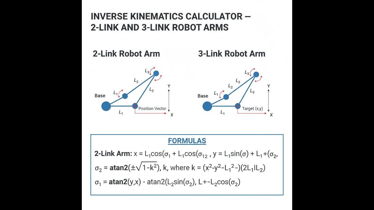
Robot Arm Kinematics Diagram

inverse kinematics interactive visualizer
Position the target crosshair and watch the robot arm calculate required joint angles in real-time. Toggle between 2-link and 3-link configurations to see how additional degrees of freedom affect reachability and control.
ANGLE θ₁
--°
ANGLE θ₂
--°
REACHABLE
YES
FIRGELLI Automations — Interactive Engineering Calculators
How to Use This Calculator
- Select the number of links — 2-link or 3-link — from the dropdown menu.
- Enter the length of each link (L₁, L₂, and L₃ if applicable) in your chosen units.
- Enter the Target X and Target Y position coordinates. For a 3-link arm, also enter the desired end-effector orientation in degrees.
- Click Calculate to see your result.
Inverse Kinematics Calculator
Mathematical Equations
2-Link Robot Arm Inverse Kinematics
For a 2-link planar robot arm, the inverse kinematics equations are:
Use the formula below to calculate joint angles for a 2-link planar robot arm.
Joint Angle 2:
θ₂ = acos((x² + y² - L₁² - L₂²) / (2L₁L₂))
Joint Angle 1:
θ₁ = atan2(y, x) - atan2(L₂sin(θ₂), L₁ + L₂cos(θ₂))
Reachability Condition:
|L₁ - L₂| ≤ √(x² + y²) ≤ L₁ + L₂
3-Link Robot Arm Inverse Kinematics
For a 3-link planar robot arm with specified end-effector orientation:
Use the formula below to calculate joint angles for a 3-link planar robot arm.
Wrist Position:
wx = x - L₃cos(φ)
wy = y - L₃sin(φ)
First Two Joint Angles (same as 2-link for wrist position):
θ₂ = acos((wx² + wy² - L₁² - L₂²) / (2L₁L₂))
θ₁ = atan2(wy, wx) - atan2(L₂sin(θ₂), L₁ + L₂cos(θ₂))
Third Joint Angle:
θ₃ = φ - θ₁ - θ₂
Simple Example
2-link arm, L₁ = 100mm, L₂ = 80mm, target position (120, 90):
- Distance to target = √(120² + 90²) = 150mm — within reach range of 20mm to 180mm.
- θ₂ = arccos((14400 + 8100 − 10000 − 6400) / 16000) = arccos(0.38125) = 67.59°
- θ₁ = atan2(90, 120) − atan2(73.95, 130.5) = 36.87° − 29.55° = 7.32°
Technical Analysis and Applications
Understanding Inverse Kinematics
Inverse kinematics is the mathematical process of determining joint angles required to position a robot's end-effector at a desired location and orientation. Unlike forward kinematics, which calculates end-effector position from joint angles, inverse kinematics works backwards from the desired position to find the required joint configurations.
This inverse kinematics calculator robot arm tool is fundamental to robotic motion planning, enabling precise control of robotic manipulators in manufacturing, automation, and research applications. The complexity increases significantly as the number of degrees of freedom grows, making calculators like this essential for engineers and roboticists.
2-Link vs 3-Link Robot Arms
A 2-link robot arm provides two degrees of freedom, allowing it to reach any point within its workspace but without control over end-effector orientation. This configuration is sufficient for many pick-and-place operations and simple material handling tasks.
A 3-link robot arm adds a third degree of freedom, typically allowing control over both position and orientation of the end-effector. This additional capability is crucial for tasks requiring specific approach angles, such as assembly operations or precise welding applications.
Workspace and Reachability
The workspace of a robot arm is defined by the geometric constraints of its link lengths. For a 2-link arm, the reachable workspace forms an annulus (ring shape) centered at the base, with inner radius |L₁ - L₂| and outer radius L₁ + L₂. Points outside this region are physically unreachable, making reachability analysis a critical component of any inverse kinematics calculator robot arm solution.
Practical Applications
Inverse kinematics calculations are essential in numerous industrial applications:
- Manufacturing Automation: CNC machines and robotic arms use inverse kinematics to follow programmed tool paths with high precision.
- Assembly Lines: Pick-and-place robots rely on these calculations to position components accurately during assembly processes.
- Welding and Cutting: Robotic welding systems require precise end-effector positioning and orientation control.
- Medical Robotics: Surgical robots use sophisticated inverse kinematics for minimally invasive procedures.
- Inspection Systems: Automated inspection equipment positions cameras and sensors using kinematic control.
In many of these applications, FIRGELLI linear actuators serve as the driving mechanism for joint movement, providing precise, reliable motion control with excellent repeatability and load capacity.
Worked Example
Consider a 2-link robot arm with L₁ = 100mm and L₂ = 80mm, tasked with reaching a target position at (120mm, 90mm):
Step 1: Check Reachability
Distance to target = √(120² + 90²) = √(14400 + 8100) = √22500 = 150mm
Minimum reach = |100 - 80| = 20mm
Maximum reach = 100 + 80 = 180mm
Since 20mm ≤ 150mm ≤ 180mm, the target is reachable.
Step 2: Calculate θ₂
cos(θ₂) = (120² + 90² - 100² - 80²) / (2 × 100 × 80)
cos(θ₂) = (14400 + 8100 - 10000 - 6400) / 16000 = 6100 / 16000 = 0.38125
θ₂ = arccos(0.38125) = 67.59°
Step 3: Calculate θ₁
k₁ = 100 + 80 × cos(67.59°) = 100 + 80 × 0.38125 = 130.5
k₂ = 80 × sin(67.59°) = 80 × 0.9244 = 73.95
θ₁ = atan2(90, 120) - atan2(73.95, 130.5) = 36.87° - 29.55° = 7.32°
Design Considerations
When designing robotic systems using inverse kinematics calculations, several factors must be considered:
Singularities: Configurations where the robot loses one or more degrees of freedom, typically occurring when links are fully extended or folded back on themselves. These positions should be avoided in motion planning.
Multiple Solutions: For many target positions, multiple valid joint configurations exist (elbow-up vs elbow-down solutions). The choice depends on factors like obstacle avoidance, joint limits, and energy efficiency.
Joint Limits: Real robots have physical constraints on joint rotation ranges. The inverse kinematics calculator robot arm must verify that calculated angles fall within these limits.
Accuracy and Precision: Computational precision affects positioning accuracy. Industrial applications often require sub-millimeter precision, demanding high-resolution calculations and feedback systems.
Advanced Considerations
Modern robotic systems often incorporate additional features beyond basic inverse kinematics:
Redundancy Resolution: For arms with more than necessary degrees of freedom, optimization criteria help select the best solution among multiple valid configurations.
Obstacle Avoidance: Path planning algorithms integrate inverse kinematics with collision detection to ensure safe operation in complex environments.
Dynamic Considerations: High-speed applications must account for joint velocities and accelerations, extending inverse kinematics to include velocity and acceleration analysis.
The integration of precise linear actuators, such as those available from FIRGELLI's extensive range, ensures that the calculated joint angles can be accurately achieved in real-world applications. These actuators provide the force, precision, and reliability necessary for demanding industrial automation tasks.
Frequently Asked Questions
📐 Browse all 1000+ Interactive Calculators →
About the Author
Robbie Dickson
Chief Engineer & Founder, FIRGELLI Automations
Robbie Dickson brings over two decades of engineering expertise to FIRGELLI Automations. With a distinguished career at Rolls-Royce, BMW, and Ford, he has deep expertise in mechanical systems, actuator technology, and precision engineering.
Need to implement these calculations?
Explore the precision-engineered motion control solutions used by top engineers.


