Distance Attenuation Interactive Calculator

If you're planning a wireless link, acoustic sensor array, or fiber run, expect one thing: signals get weaker as they travel, and guessing too low on losses will end up limiting your real-world range. This Distance Attenuation Calculator lets you estimate received power, total loss, how far you can actually reach, or how much transmitter power you really need. Just plug in distance, frequency, and the attenuation coefficient for your medium. This isn't just a radio problem—it's the same story in industrial ultrasound, medical imaging, and satellite work. The page covers the core equations, a practical industrial example, a straightforward breakdown of both types of loss (free-space and in-material), and a detailed FAQ.

What is distance attenuation?

Distance attenuation is just the drop in signal strength as it travels away from the source—radio, sound, or light. The further the signal goes, the more it spreads out physically, and the more the material around it can sap energy along the way.

Simple Explanation

Picture shining a flashlight into a dark room. Close up, you get a bright spot; further away, that same light has to cover a bigger area, so any given spot will seem dimmer. That’s just spreading out. Now shine it through fog—the beam not only spreads, but the fog actually absorbs and scatters the light, so the brightness falls off faster. Distance attenuation is just both of those effects at work: spreading and absorption.

📐 Browse all 1000+ Interactive Calculators

Attenuation Diagram

Distance Attenuation Calculator

How to Use This Calculator

1. Select your calculation mode from the dropdown — received power, path loss, max distance, required transmit power, attenuation coefficient, or frequency-dependent loss.
2. Enter your transmitted power (dBm), distance (meters), frequency (MHz), and attenuation coefficient (dB/m) in the input fields shown for your selected mode.
3. Adjust any additional inputs that appear for your chosen mode, such as minimum receiver sensitivity or reference frequency.
4. Click Calculate to see your result.

<> Embed this calculator → <> Embed this animation calculator →

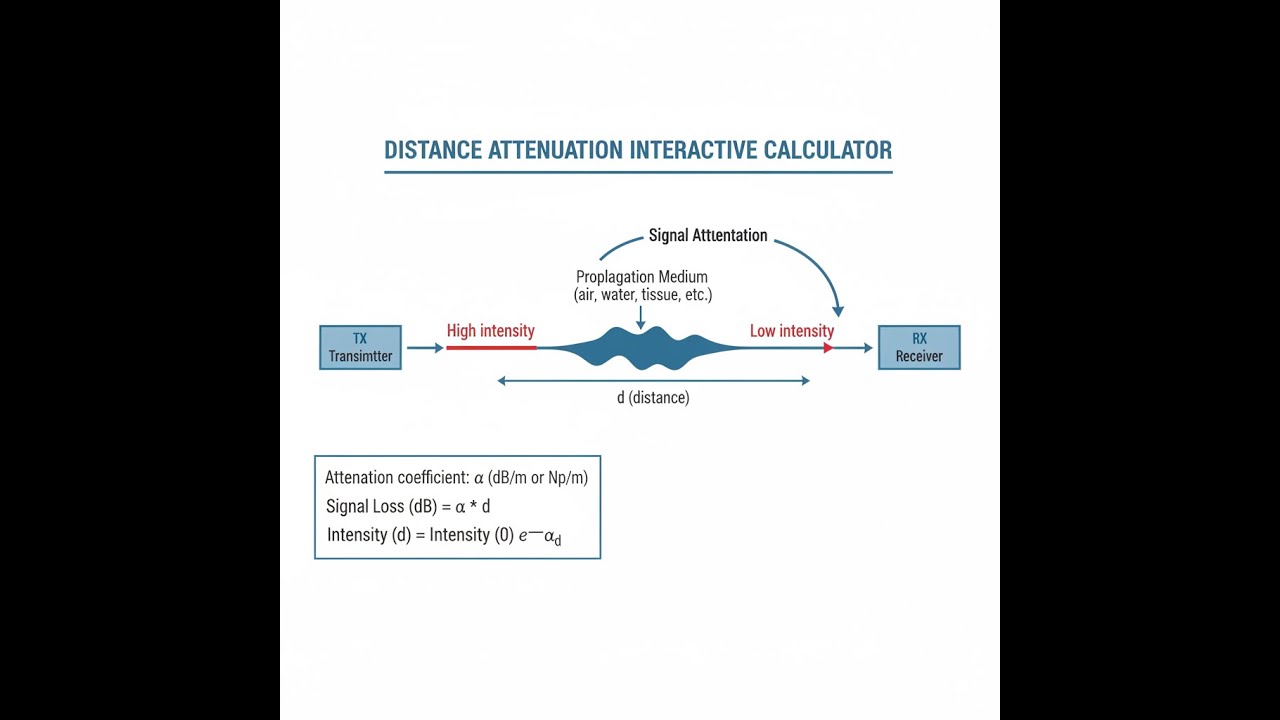
Distance Attenuation Equations

The formula below is used for free-space path loss calculations.

This formula is used for losses from absorption in the medium itself.

This sums up the whole link’s loss (including connectors, cable, and other real losses).

To factor in antenna gains for a full link budget, use this form:

Simple Example

Transmit power P₀ = 30 dBm, distance d = 100 m, frequency f = 900 MHz, attenuation coefficient α = 0.05 dB/m.

• Free-space path loss: L_FSL = 32.45 + 20 log₁₀(900) + 20 log₁₀(0.1) = 71.53 dB
• Medium attenuation: L_medium = 0.05 × 100 = 5 dB
• Total loss: 71.53 + 5 = 76.53 dB
• Received power: 30 − 76.53 = −46.53 dBm — a strong, usable signal.

Theory & Practical Applications of Distance Attenuation

Any real wave—electromagnetic or acoustic—loses strength as it moves away from its source. Two main things drive this: geometric spreading (signals get weaker just by spreading out), and absorption by whatever medium they pass through. While textbooks split these up, practical engineering (RF, sonar, medical ultrasound) pretty much always requires looking at both for realistic system predictions.

The Physics of Geometric Spreading

Free-space path loss comes from the fact that as a signal radiates outward, it covers the surface of a bigger and bigger sphere—the power per unit area goes down with 1/d² (the inverse-square law). That’s true even if there’s zero absorption. Engineers translate that law to dB using the log form—makes it easy to add up all the gains and losses in a system.

One step that often gets missed is that free-space loss itself depends on frequency. It isn’t because higher frequencies get eaten up by space (they don’t); it’s really about how antennas work. Receiving antennas pick up less energy as frequency rises (their effective area goes as wavelength squared), so a 5 GHz link will lose 6 dB more than 2.5 GHz at the same distance, just from this effect. This is why higher-frequency systems give you more bandwidth and smaller antennas, but at the cost of much shorter useful range or needing more transmit power. For example, 5 GHz WiFi won’t reach nearly as far as 2.4 GHz using the same setup—even if your data rate is higher.

Medium-Dependent Exponential Attenuation

Spreading isn’t the only source of loss—real-world materials absorb and scatter some energy as the wave goes through. That’s where the attenuation coefficient (α) comes in: it combines true absorption and scattering. Unlike geometric loss scaling as 20 log(d), absorption adds up in direct proportion to distance: L_medium = α × d. If you’re working somewhere with lossy media, this can easily become your main limitation, not the spreading loss.

Microwave links show the effect clearly: certain frequencies (like 22.2 GHz for water vapor, 60 GHz and 118.75 GHz for oxygen) are seriously attenuated due to molecular resonances. Rain is another frequent culprit—in heavy weather, you can lose 10-50 dB over a satellite or terrestrial link, depending on frequency and path length. In optical fiber, the best wavelength to run glass is 1.55 μm (0.2 dB/km loss) for exactly this reason—trying to push signals further at 1.3 μm already adds 75% more attenuation. Over a 100 km fiber route, this difference alone stacks up 20 dB more loss, before you even count splices.

In buildings, attenuation gets tied to both frequency and the construction materials. At 900 MHz, a concrete wall might only cause half a dB per meter; at 60 GHz, it jumps to 15 dB/m, or more. For ordinary drywall, you’ll typically see 3-5 dB loss at 2.4 GHz per wall, but 5 GHz can drop twice as much through the same partition. For real problematic materials like Low-E glass, even higher frequencies (28, 39 GHz, as used for 5G) don’t get through at all. Lower frequencies (like 225–400 MHz, used for public service radios) penetrate buildings pretty well, but require much bulkier antennas.

Worked Example: Industrial Wireless Sensor Network Design

If you’re building a wireless sensor network in a factory with concrete walls and steel rebar, your working range is never just what the “spec sheet” says. Let’s take a typical problem: you need 200 meters range from a sensor to a gateway, through concrete and metal clutter.

Given Parameters:

• Sensor transmit power: P₀ = +10 dBm (10 mW)
• Gateway receiver sensitivity: -95 dBm minimum
• Frequency: 900 MHz (not too bulky an antenna, not too bad at getting through walls)
• Margin: 20 dB (covers fading, interference, aging, the unknowns)
• Concrete walls: α = 0.8 dB/m, walls are 0.25 m thick, there are 3
• Antenna gain: +2 dBi (sensor), +5 dBi (gateway directional)

Step 1: Allowable path loss

Link budget = P_t + G_t + G_r – receiver sensitivity – margin = 10 + 2 + 5 – (-95) – 20 = 92 dB

Step 2: Free-space path loss (200 m)

L_FSL = 32.45 + 20 log₁₀(900) + 20 log₁₀(0.2) = 77.55 dB

Step 3: Walls loss

Each wall: 0.8 × 0.25 = 0.2 dB. Three walls: 0.6 dB total.

Step 4: Extra loss (clutter and machinery)

Metal all around will cause multipath and fading plus general clutter. 8 dB is a practical estimate, based on actual industrial site trials.

Step 5: Total up and compare

L_total = 77.55 + 0.6 + 8 = 86.15 dB
Available = 92 dB → spare margin = 5.85 dB

Step 6: Reality check

5.85 dB isn’t much security in a harsh environment where seasonal changes, power supply dips, and corroded connectors can sap more margin over time. To shore up reliability:

• Raise sensor output to +17 dBm (adds 7 dB, still legal for ISM band)
• Put the gateway up higher to clear clutter (cuts clutter loss by 3 dB)
• Add forward error correction with 6 dB effective coding gain

New margin: 5.85 + 7 + 3 + 6 = 21.85 dB—enough for long-term operation with something left for the unexpected.

Atmospheric and Weather Effects on RF Propagation

Above 10 GHz, the air itself can become a big source of loss, varying a lot by weather. Some frequencies take a beating due to water vapor or oxygen; others are “windows” with far less loss. Rain, especially on satellite or long microwave links, is often the limiting factor. There are practical tradeoffs: a 100 km path at 12 GHz in moderate rain may lose 12 dB, but can go up to 45 dB at 30 GHz. Operators have to add power margin, use lower rates, or deploy several sites to keep a service working in bad weather. Some ITU models help estimate likely outage and how much extra margin you'll need above just the clear-sky loss.

Application in Medical Ultrasound Imaging

Acoustic loss in tissue increases with frequency. For medical imaging, this puts you between two realities—lower frequencies dive deeper but blur out detail, while high frequencies give crisp images but barely penetrate. At 3.5 MHz, you reach around 15 cm deep (just enough for an abdomen scan) but can’t resolve below half a millimeter. At 15 MHz, you’ll only see a few centimeters in, but can resolve vessels and tiny structures. Bone and air block sound even harder. Bone can lose 30-40 dB at diagnostic frequencies in just a centimeter of skull. That’s why “ultrasound windows” are chosen carefully, and why coupling gel is always used for surface scans—without it, you lose almost everything to reflection.

Fiber Optic Attenuation Engineering

Losses in optical fibers mostly come from scattering (which drops steeply with increasing wavelength) and absorption (which rises in the infrared). That leaves a “minimum spot” near 1.55 μm, where modern fiber gets 0.2 dB/km loss. Submarine cables run amplifiers every 50–80 km to offset this loss; even then, a 10,000 km cable stacks up to 2000 dB loss, so dozens of amplifiers keep the signal above the noise. For even longer runs, Raman amplification can pull the effective loss to 0.15 dB/km if done well, but dispersion and nonlinear effects start to be the limitations, not just plain attenuation.

Practical Considerations for Link Budget Analysis

All these equations are averages. Out in the field, unpredictable things—people moving, weather, aging hardware—make fades and drops worse than theory. That’s why systems always add significant “margin” on top of calculated loss. Multipath (from movement or reflections) can swing signal 20–30 dB in just a few centimeters. Buildings and terrain create shadow fades that can run 6–12 dB up and down. Put together, you need margins of 30–40 dB beyond the textbook value for reliable wireless in tough environments. Temperature shifts, cable and connector aging, and even rain can nick away another few dB over the years, so build those into your initial plan if you want equipment not to fail quietly six months after install.

For more calculators on RF, ultrasound, and optic propagation, visit the FIRGELLI Engineering Calculator Hub.

Frequently Asked Questions