If you don’t account for friction loss when sizing pipes, you’ll probably end up with a pump that’s too small, lower-than-expected flow, and a pile of change orders after you’ve installed everything. The Darcy-Weisbach calculator below handles head loss, pipe diameter, flow velocity, friction factor, flow rate, or required length — all based on actual pipe details and fluid properties. You’ll rely on this whether you’re laying out an HVAC loop, a city water main, a process line in a chemical plant, or a crude oil pipeline. Below, you’ll find the core equations, a practical water system example, flow regime basics, and a focused FAQ.
What is the Darcy-Weisbach equation?
The Darcy-Weisbach equation gives you the pressure or head you lose from friction as fluid moves through pipe. Put in the pipe’s length, diameter, velocity, and its friction factor — you get the extra energy your pump will need simply to keep stuff moving.
Simple Explanation
Picture forcing water through a garden hose: the longer the hose, the smaller its diameter, and the faster you try pushing water through, the more it pushes back on your supply. The Darcy-Weisbach equation quantifies that resistance — called “friction head loss” — letting you pick real-world sizes for pumps or pipes before you buy anything or start digging.
📐 Browse all 1000+ Interactive Calculators
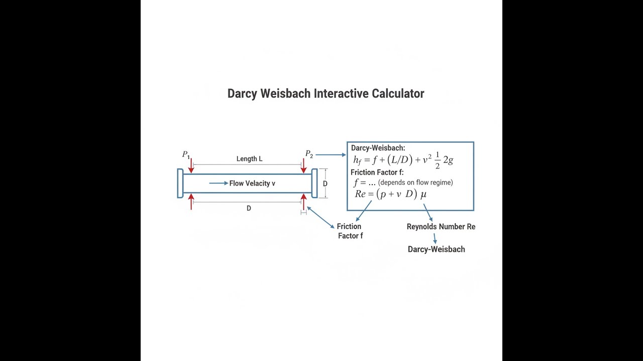
System Diagram

Interactive Calculator
How to Use This Calculator
This calculator is intended for education, concept evaluation, and preliminary design. Results are based on the equations and assumptions described on this page, but cannot account for every real-world load case, tolerance, material property, environmental condition, installation detail, safety factor, code, or regulatory requirement. Verify all inputs, assumptions, units, and results independently before selecting components or using the result in a real application. Safety-critical, structural, medical, lifting, transportation, or regulated applications must be reviewed by a qualified engineer.
- Pick which variable you want to solve for in the Calculation Mode dropdown: head loss, pipe diameter, velocity, friction factor, flow rate, or length.
- Enter known values into the relevant fields: friction factor, length, diameter, velocity, viscosity, pipe roughness as needed.
- If your mode needs a head loss or a flow rate as an input, plug those in as well.
- Click Calculate to get your result.
Darcy-Weisbach interactive visualizer
See how friction factor, pipe size, and flow velocity combine to drive up head loss. Adjust the sliders and you’ll instantly see how much pressure drop and energy cost you’re adding or saving.
HEAD LOSS
5.10 m
REYNOLDS
200,000
PRESSURE
50 kPa
FIRGELLI Automations — Interactive Engineering Calculators
Governing Equations
Here’s the core formula for friction losses in pipe flow.
Darcy-Weisbach Equation
hf = f · (L / D) · (v² / 2g)
Where:
- hf = head loss due to friction (m)
- f = Darcy friction factor (dimensionless)
- L = pipe length (m)
- D = pipe diameter (m)
- v = mean flow velocity (m/s)
- g = gravitational acceleration (9.81 m/s²)
Reynolds Number
Re = (v · D) / ν
Where:
- Re = Reynolds number (dimensionless)
- ν = kinematic viscosity (m²/s)
Flow regimes: Laminar (Re < 2300), Transitional (2300 ≤ Re ≤ 4000), Turbulent (Re > 4000)
Pressure Drop
ΔP = ρ · g · hf
Where:
- ΔP = pressure drop (Pa)
- ρ = fluid density (kg/m³, typically 1000 kg/m³ for water)
Volumetric Flow Rate
Q = v · A = v · (π · D² / 4)
Where:
- Q = volumetric flow rate (m³/s)
- A = pipe cross-sectional area (m²)
Relative Roughness
ε/D = ε / D
Where:
- ε = absolute pipe roughness (m)
- ε/D = relative roughness (dimensionless)
Simple Example
Given: f = 0.02, L = 100 m, D = 100 mm (0.1 m), v = 2 m/s, g = 9.81 m/s²
Formula: hf = f · (L/D) · (v²/2g)
Calculation: hf = 0.02 × (100/0.1) × (4/19.62)
Result: hf = 0.02 × 1000 × 0.204 = 4.08 m
Theory & Practical Applications
The Darcy-Weisbach equation gives you direct, practical numbers for energy loss in pipe flow, regardless of fluid or pipe material. Unlike rough estimates such as Hazen-Williams (which only works for cold water), Darcy-Weisbach applies to any Newtonian fluid and pipe size. That’s why everyone from chemical plants to city utilities uses it for anything beyond early project sketches.
Fundamental Physics and Flow Regimes
Darcy-Weisbach links mechanical energy losses to viscous drag and turbulence inside the pipe. The friction factor f isn’t just a look-up value — it reflects everything from how smooth the inside of your pipe is to what the flow is doing near the wall. In laminar flow (Re < 2300), f is just 64 divided by Reynolds number. Surface roughness doesn’t matter here because fluid moves in smooth, non-interacting layers, so wall bumps aren’t “felt.”
The transition regime (2300–4000) is trouble for design: this is an unstable range where small disruptions trigger bursts of turbulence. Avoid running systems here. The friction factor becomes jumpy, and things like small valve adjustments or a change in fluid temperature can swing everything.
Municipal water pipes almost always run with turbulent flow (Re higher than 100,000). On the other hand, lines for sticky fluids in processing plants might have intentionally slow, laminar flow to limit mixing.
The Moody Diagram and Implicit Friction Factor Determination
Turbulent flow friction factors come from the Colebrook-White equation (or the Moody diagram), and you can’t just write the answer in one step — the equation is implicit. Historically, engineers used the Moody chart for quick guesses. Today’s calculators do the iterations, but you need to understand what the chart shows. At very high Re and if your pipe is rough, the friction factor stops changing when you go faster (lines get flat). That means pumping harder won’t drop friction losses any farther — you’re limited by roughness, not viscosity. This comes up a lot for old or corroded pipes.
The practical side: Say you’re picking between steel and PVC for a 150 mm water pipe. Steel’s roughness is about 0.045 mm, so ε/D = 0.0003. PVC is much smoother (ε/D ≈ 0.00001). At Re = 500,000, the steel pipe needs about 34% more pump power for the same flow than PVC. That extra power, over decades, outweighs the initial cost savings on pipe material most of the time.
Scale Effects and the Economic Pipe Diameter Problem
The head loss by Darcy-Weisbach scales as v²/D, but if you express flow as Q, you see that doubling pipe diameter lowers velocity by four times (for the same Q), and friction loss drops by 32 times. This is the main economic lever in distribution design: bigger pipes cost more at first, but they cut down on power bills sharply. The “best” diameter is the one where the capital cost of bigger pipe balances out against the years of energy savings — for water, typical velocities end up around 1.5–3.0 m/s because of this trade-off.
On big jobs like the Trans-Alaska oil pipeline (about 1,200 mm diameter, 1,300 km long), designers chose the size to keep head loss and the number of expensive pump stations down. If they’d picked a pipe one size smaller, it would have meant adding multiple new pump stations and tripling the energy bill, purely because of how friction loss cube-scales with smaller pipe and higher velocity.
Industrial Applications Across Engineering Domains
In HVAC, Darcy-Weisbach is useful for sizing supply ducts and picking air handler fans. Typical duct velocities of 6–10 m/s represent the balance between noise (faster is noisier) and how much room the ducts take up overhead (slower flows need bigger ducts). In a commercial building, friction losses can eat up a big chunk of your fan pressure.
In chemical processing, the equation is key for getting slurry or catalyst lines right. If fluid temperature drops, viscosity can double and suddenly head loss jumps by a quarter — which can cause flow to collapse and shut down a production line if you don’t have extra pump margin or good flow controls.
Worked Example: Municipal Water Distribution System Design
Let’s say you’re laying out a water main to supply a subdivision, and you’re deciding between 400, 450, and 500 mm ductile iron pipe. You need to deliver 315 L/s through 2.4 km. Different pipe sizes give you different velocities, Reynolds numbers, friction factors, and ultimately different energy costs over 20+ years.
Step 1: Calculate flow velocities for each diameter option
For 400 mm: v = 0.315 / 0.1257 = 2.506 m/s
For 450 mm: v = 0.315 / 0.1590 = 1.981 m/s
For 500 mm: v = 0.315 / 0.1963 = 1.604 m/s
Step 2: Determine Reynolds numbers and flow regimes
(Kinematic viscosity for water at 20°C = 1.0×10⁻⁶ m²/s)
400 mm: Re = 1,002,400 (turbulent)
450 mm: Re = 891,450 (turbulent)
500 mm: Re = 802,000 (turbulent)
Step 3: Calculate relative roughness and friction factors
400 mm: ε/D = 0.00065 (f ≈ 0.0192)
450 mm: ε/D = 0.00058 (f ≈ 0.0188)
500 mm: ε/D = 0.00052 (f ≈ 0.0185)
Step 4: Apply Darcy-Weisbach equation to calculate head losses
400 mm: hf = 36.89 m
450 mm: hf = 20.07 m
500 mm: hf = 11.65 m
Step 5: Calculate pressure drops and pumping power requirements
(Water, ρ = 1000 kg/m³, pump eff. 75%)
400 mm: Power = 152.0 kW
450 mm: Power = 82.7 kW
500 mm: Power = 48.0 kW
Step 6: Economic analysis and selection
If power is $0.12/kWh and you run 6,000 hours per year at this flow:
400 mm: annual energy $109,440
450 mm: annual energy $59,544
500 mm: annual energy $34,560
Over 20 years, the big pipe saves about $950,000 in energy, which usually dwarfs initial pipe installation cost differences. Choosing a slightly bigger line can be the difference between profit and pain on a municipal system, especially as pipe roughness increases with age (from corrosion or scale), which raises head loss proportionally more in small-diameter pipes.
Advanced Considerations and Limitations
The basic Darcy-Weisbach setup assumes straight, round, steady-flow pipes. Real systems include elbows, tees, reducers, and valves — all adding local (“minor”) losses. For complex layouts, you need to add up those K-factors or use equivalent length methods. In some cases, minor losses are actually bigger than the loss from the straight-pipe run itself, so don’t skip them in calculations.
If you’re moving non-Newtonian fluids (think slurries or polymer solutions), the standard friction factor equations break down. You’ll need fluid-specific correlations or experimental data if you want numbers you can trust. For anything past clean water or mineral oil, don’t just plug and chug with textbook f equations.
For more engineering tools, check the FIRGELLI Engineering Calculator Library.
Frequently Asked Questions
Free Engineering Calculators
Explore our complete library of free engineering and physics calculators.
Browse All Calculators →🔗 Explore More Free Engineering Calculators
- Pipe Flow Velocity Calculator
- Reynolds Number Calculator — Laminar or Turbulent
- Hydraulic Pump Flow Rate Calculator
- Cylinder Volume Calculator — Tank Pipe Capacity
- Cv Flow Calculator
- Darcys Law Calculator
- Mean Free Path Calculator
- Friction Force Calculator — Static and Kinetic
- Water Hammer Pressure Calculator
- Projectile Motion Calculator
About the Author
Robbie Dickson — Chief Engineer & Founder, FIRGELLI Automations
Robbie Dickson brings over two decades of engineering expertise to FIRGELLI Automations. With a distinguished career at Rolls-Royce, BMW, and Ford, he has deep expertise in mechanical systems, actuator technology, and precision engineering.
Video Walkthrough - How to Use This Calculator
Need to implement these calculations?
Explore the precision-engineered motion control solutions used by top engineers.


