Demand variability and supplier lead time uncertainty are the 2 biggest causes of stockouts — and guessing your buffer inventory is expensive either way. Use this Safety Stock Statistical Calculator to calculate optimal buffer inventory levels using service level targets, demand standard deviation, and lead time inputs. Getting this right matters in manufacturing, distribution, and retail, where a stockout can halt a production line or lose a customer permanently. This page covers the formulas, a worked example, the underlying statistical theory, and a full FAQ.
What is Safety Stock?
Safety stock is extra inventory you hold above your expected demand during the time it takes for a new order to arrive. It acts as a buffer against demand spikes and supplier delays so you don't run out of stock.
Simple Explanation
Think of safety stock like a spare tire. You don't expect to need it, but when demand runs hotter than average or your supplier is late, it's what keeps operations moving. The more unpredictable your demand or your supplier's delivery time, the bigger that spare tire needs to be.
📐 Browse all 1000+ Interactive Calculators
How to Use This Calculator
- Select your calculation mode — Basic Safety Stock, Variable Lead Time, Reorder Point, or one of the reverse-solve modes.
- Enter your average demand, standard deviation of demand, average lead time, and service level (or safety stock, depending on mode).
- If using Variable Lead Time mode, also enter the standard deviation of lead time.
- Click Calculate to see your result.
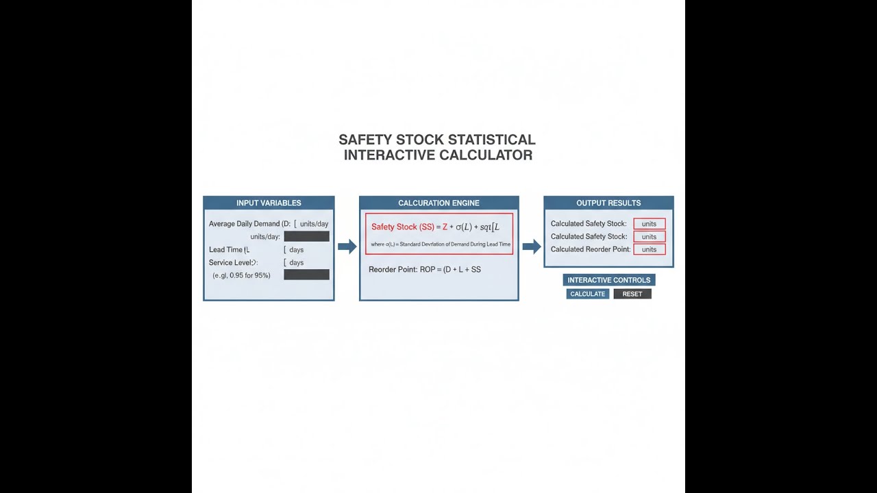
Diagram

Safety Stock Statistical Calculator
Safety Stock Statistical Interactive Calculator
Calculate optimal buffer inventory levels using service level targets, demand standard deviation, and lead time variability. Visualize how demand uncertainty and supplier delays impact your required safety stock buffer.
SAFETY STOCK
65 units
Z-SCORE
1.645
REORDER POINT
765 units
STOCKOUT RISK
5.0%
FIRGELLI Automations — Interactive Engineering Calculators
Equations & Formulas
Use the formula below to calculate basic safety stock with constant lead time.
Basic Safety Stock (Constant Lead Time)
SS = Z × σD × √LT
Where:
SS = Safety Stock (units)
Z = Z-score corresponding to desired service level (dimensionless)
σD = Standard deviation of demand (units per period)
LT = Lead time (periods)
Use the formula below to calculate safety stock when both demand and lead time vary.
Variable Demand and Variable Lead Time
SS = Z × √(LTavg × σD2 + Davg2 × σLT2)
Where:
Z = Z-score for service level (dimensionless)
LTavg = Average lead time (periods)
σD = Standard deviation of demand (units per period)
Davg = Average demand (units per period)
σLT = Standard deviation of lead time (periods)
Use the formula below to calculate the reorder point from average demand, lead time, and safety stock.
Reorder Point
ROP = (Davg × LTavg) + SS
Where:
ROP = Reorder Point (units)
Davg = Average demand (units per period)
LTavg = Average lead time (periods)
SS = Safety Stock (units)
Use the formula below to calculate the standard deviation of total demand accumulated over the lead time period.
Standard Deviation During Lead Time
σLT = σD × √LT
Where:
σLT = Standard deviation during lead time (units)
σD = Standard deviation of daily demand (units per period)
LT = Lead time (periods)
Simple Example
Average daily demand: 100 units
Standard deviation of demand: 20 units/day
Average lead time: 7 days
Target service level: 95% → Z-score = 1.645
σ during lead time = 20 × √7 = 52.92 units
Safety Stock = 1.645 × 52.92 = 87.06 units
Theory & Engineering Applications
Safety stock represents the buffer inventory maintained above expected demand during lead time to protect against demand variability, supply uncertainty, and forecast errors. Unlike deterministic inventory models that assume perfect predictability, statistical safety stock calculations explicitly incorporate probabilistic distributions to quantify risk and establish optimal service levels. This approach transforms inventory management from reactive fire-fighting to proactive risk mitigation grounded in quantitative analysis.
Fundamental Statistical Principles
The core assumption underlying most safety stock calculations is that demand follows a normal distribution during the replenishment lead time. This assumption, while imperfect, provides a tractable framework for analysis and works reasonably well for products with stable, high-volume demand patterns. The Z-score represents the number of standard deviations above the mean demand required to achieve a target service level. For instance, a 95% service level corresponds to a Z-score of 1.645, meaning safety stock must cover demand up to 1.645 standard deviations above average to achieve a 5% stockout probability.
A critical but often overlooked aspect is the distinction between demand variability and forecast error. Standard deviation of demand (σD) captures inherent randomness in customer orders, while forecast error represents systematic bias or model inadequacy. Many practitioners mistakenly use forecast error variance directly in safety stock formulas, which double-counts variability and leads to excessive inventory. The proper approach separates these components: safety stock addresses random variation, while forecast bias requires model improvement or adjustment factors.
Variable Lead Time Complexity
When lead time itself varies, the safety stock calculation becomes significantly more complex because uncertainty now exists in both dimensions. The combined variance formula accounts for this interaction: variance during lead time equals the product of average lead time and demand variance, plus the product of average demand squared and lead time variance. This multiplicative relationship reveals a non-obvious insight: for products with high average demand, lead time variability contributes disproportionately to total uncertainty. A semiconductor manufacturer with 10,000 units/day average demand and 2-day lead time standard deviation faces vastly different risk than a specialty chemical supplier with 100 units/day and the same lead time variability.
The mathematical derivation assumes independence between demand and lead time, which may not hold in practice. Supplier capacity constraints can create positive correlation: when demand spikes, suppliers struggle to maintain normal lead times. Incorporating this correlation requires advanced time-series analysis or simulation, moving beyond closed-form solutions. Organizations facing correlated variability should consider increasing safety stock by 15-30% beyond the standard formula as a pragmatic adjustment.
Service Level Interpretation and Cost Trade-offs
Service level definition varies across industries, creating confusion. Cycle service level (CSL) represents the probability that all demand during a replenishment cycle is satisfied without stockout. Fill rate measures the fraction of total demand met from stock. These metrics diverge significantly for low-volume, high-variability items. A 95% cycle service level might correspond to only an 85% fill rate for sporadic demand patterns. Safety stock calculations typically target CSL, but executives often care more about fill rate, creating misalignment between inventory policies and business objectives.
The optimal service level balances carrying costs against stockout costs. While textbooks present elegant economic order quantity (EOQ) extensions incorporating shortage costs, real-world implementation faces two fundamental challenges. First, stockout costs are notoriously difficult to quantify—they include lost sales, expediting expenses, production disruptions, and intangible customer goodwill erosion. Second, service level decisions rarely happen at the SKU level; corporate policies mandate broad targets (e.g., "95% for A-items") without granular cost analysis. Progressive organizations segment inventory using ABC-XYZ classification, applying higher service levels to critical, predictable items and accepting lower targets for erratic, low-value SKUs.
Practical Calculation Example: Medical Device Distribution
Consider a regional medical device distributor managing inventory of surgical staplers. Historical data shows average daily demand of 87 units with a standard deviation of 23 units. The supplier in Taiwan provides an average lead time of 42 days with a standard deviation of 6 days. The company targets a 98% service level to minimize surgical procedure delays.
Step 1: Determine Z-score
For a 98% service level, Z = 2.054 (from standard normal distribution tables)
Step 2: Calculate combined variance during lead time
VarianceLT = (LTavg × σD2) + (Davg2 × σLT2)
VarianceLT = (42 × 232) + (872 × 62)
VarianceLT = (42 × 529) + (7569 × 36)
VarianceLT = 22,218 + 272,484
VarianceLT = 294,702 units2
Step 3: Calculate standard deviation during lead time
σLT = √294,702 = 542.87 units
Step 4: Calculate safety stock
SS = Z × σLT
SS = 2.054 × 542.87
SS = 1,115.05 ≈ 1,115 units
Step 5: Calculate reorder point
Average demand during lead time = 87 units/day × 42 days = 3,654 units
ROP = 3,654 + 1,115 = 4,769 units
Interpretation: The distributor should maintain 1,115 units of safety stock and reorder when inventory falls to 4,769 units. This policy provides 98% protection against stockouts, balancing the high cost of surgical delays against inventory carrying costs. Notice that lead time variability contributes 272,484 out of 294,702 total variance units—92% of the total uncertainty. Supplier lead time reduction initiatives would dramatically reduce required safety stock; reducing σLT from 6 to 3 days would cut safety stock by approximately 35%.
Advanced Considerations in Modern Supply Chains
Traditional safety stock formulas assume stationary demand—constant mean and variance over time. Modern supply chains face non-stationary demand with trends, seasonality, and structural breaks. Pharmaceutical companies launching new drugs experience exponential growth; consumer electronics face product lifecycle decay. Applying static safety stock calculations to growing products systematically underestimates required buffer, while declining products accumulate excess inventory. Time-varying safety stock policies adjust the standard deviation window, using only recent data for trending items while longer histories work for stable products.
Multi-echelon inventory optimization (MEIO) revolutionized safety stock placement by recognizing that holding buffer at multiple supply chain stages provides redundant protection. A distribution network with regional warehouses and retail stores traditionally maintained safety stock at every location. MEIO models optimize total network safety stock by concentrating buffers at strategic locations—typically central facilities—while reducing downstream safety stock. This risk pooling effect exploits the statistical principle that aggregated demand variance grows slower than linear scaling, often reducing total inventory by 20-40% while maintaining or improving service levels. To learn more about optimizing calculations across engineering applications, visit our complete engineering calculator library.
Practical Applications
Scenario: Automotive Parts Supplier During Supply Chain Disruption
Marcus, a supply chain manager at a tier-2 automotive parts supplier, faces increasing lead time variability from their Chinese fastener vendor due to port congestion. Historical data showed 21-day average lead time with 3-day standard deviation, but recent shipments range from 18 to 35 days. Average daily demand is 4,200 fasteners with 680-unit standard deviation. Using the variable lead time calculator mode with 95% service level, he calculates a safety stock requirement of 8,347 units compared to the previous 5,462 units—a 53% increase. This analysis helps Marcus justify additional warehouse space and negotiate higher pricing with customers to cover increased working capital costs. More importantly, it quantifies the financial impact of supplier reliability, supporting his business case for dual-sourcing despite 8% higher piece prices from a domestic supplier.
Scenario: Pharmaceutical Distribution Service Level Optimization
Dr. Anita Patel, operations director for a specialty pharmaceutical distributor, reviews safety stock policies for their oncology drug portfolio. One critical medication costs $12,400 per vial with monthly carrying costs of 2.5% (equivalent to 30% annually). Current policy maintains 99.5% service level requiring 287 vials safety stock, representing $3.56 million in working capital. By using the service level calculation mode with current inventory levels, she discovers this translates to tolerating only 1.8 stockouts per year. After consulting clinical partners, she learns that a 48-hour delay can be managed through alternative treatments or emergency overnight shipments costing $850 per incident. Reducing service level to 98% cuts safety stock to 198 vials, freeing $1.1 million in capital while accepting approximately 7 stockouts annually costing $5,950 total—a dramatic improvement in total cost while maintaining acceptable patient care standards.
Scenario: E-commerce Retailer Seasonal Inventory Planning
Jennifer, inventory planning manager for an online home goods retailer, prepares for back-to-school season where demand patterns become highly volatile. A popular desk organizer normally sells 340 units/day (σ = 52 units) with 14-day lead time from their Vietnam supplier. During the six-week back-to-school peak, demand jumps to 890 units/day but standard deviation increases to 267 units as order patterns become erratic. Using the reorder point calculator at 95% service level, she determines peak season requires a reorder point of 17,321 units versus off-season 2,180 units. This calculation reveals the futility of increasing standing orders linearly with demand—the reorder point increases nearly 8x due to compounding variability effects. Jennifer implements a pre-positioning strategy, building 12,000 units of buffer inventory before the season starts to avoid constant expediting. Post-season analysis shows this approach reduced logistics costs by $23,400 compared to reactive replenishment while avoiding any stockouts during the critical selling window.
Frequently Asked Questions
Free Engineering Calculators
Explore our complete library of free engineering and physics calculators.
Browse All Calculators →🔗 Explore More Free Engineering Calculators
About the Author
Robbie Dickson — Chief Engineer & Founder, FIRGELLI Automations
Robbie Dickson brings over two decades of engineering expertise to FIRGELLI Automations. With a distinguished career at Rolls-Royce, BMW, and Ford, he has deep expertise in mechanical systems, actuator technology, and precision engineering.
Need to implement these calculations?
Explore the precision-engineered motion control solutions used by top engineers.


