Coefficient Of Discharge Interactive Calculator

If you’re sizing hydraulic systems, picking a flow meter, or working out nozzle calibration, you know the numbers you get from theory rarely match what you see in real flow tests. This Coefficient of Discharge Calculator lets you quickly work out Cd, actual flow rate, orifice area, velocity, required head, or theoretical flow rate given the usual inputs (orifice area, head, known discharge, etc). If you get Cd wrong in water, aerospace, or chemical applications, you risk shorting fuel, over-pressurizing a line, or miscalculating flow. Below is a breakdown of the equations, a worked hydraulic example, explanations of phenomena like vena contracta and Reynolds effects, and some direct Q&A.

What is Coefficient of Discharge?

The Coefficient of Discharge (Cd) tells you how much real flow you get through an opening versus the ideal, lossless prediction. So if Cd is 0.62, your actual flow is only 62% of what you'd expect if there were no friction or losses at all.

Simple Explanation

If you’ve tried blowing through a straw compared to a big tube, you know most of the resistance comes from turbulence, friction, and the way flow pinches down as it exits. Cd measures exactly that: how much the real-world effects pull your output below the perfect-physics number. A value close to 1.0 means your orifice or nozzle hardly restricts the flow.

📐 Browse all 1000+ Interactive Calculators

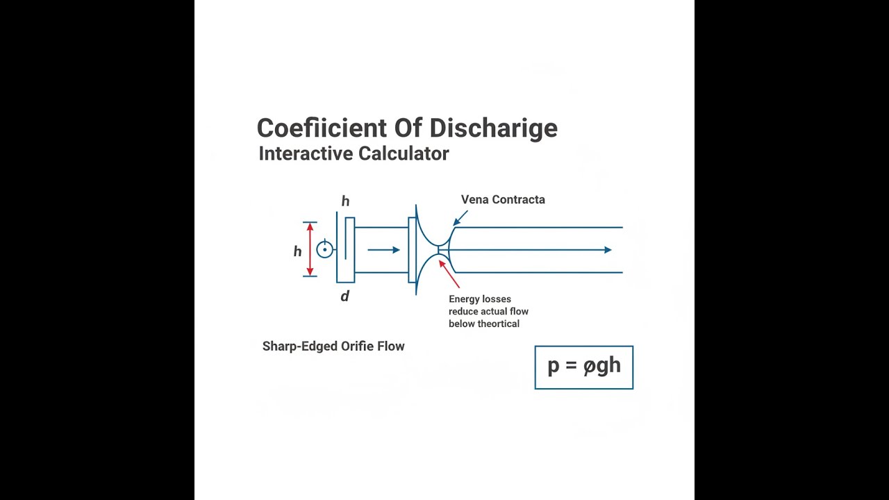
Flow Through Orifice Diagram

Interactive Calculator

How to Use This Calculator

1. Pick what you want to solve for (Cd, actual flow, area, velocity, head, or theoretical flow) using the dropdown.
2. Provide the required inputs for your chosen mode. Inputs change depending on the selected calculation.
3. Check the gravity value matches your project (default is 9.81 m/s², adjust if needed for unusual environments).
4. Click Calculate to view your answer.

<> Embed this calculator → <> Embed this animation calculator →

Governing Equations

Here's the practical equation you’ll use for Cd, and how it fits into real flow:

Simple Example

If you have a sharp-edged orifice of 0.01 m², 2 m below the water line, the calculation is straightforward: Theoretical velocity = √(2 × 9.81 × 2) = 6.26 m/s. So theoretical flow = 0.01 × 6.26 = 0.0626 m³/s. At Cd = 0.62, your actual flow is 0.62 × 0.0626 = 0.0388 m³/s.

Theory & Practical Applications

Physical Mechanisms Governing Discharge Coefficient

The drop in flow you see at an orifice is mostly due to three physical factors: First, the vena contracta effect causes the jet to narrow right after the orifice, so the effective area for flow is less than the hole you drilled—typically about 62–64% for a sharp edge. This is your contraction coefficient (Cc). Second, viscous boundary layer losses slow the fluid along the wall and reduce average velocity—that’s your velocity coefficient (Cv). Cd is just Cc times Cv. If your flow is fully turbulent (Re > 10,000) and the edge is sharp, Cc ≈ 0.64 and Cv ≈ 0.97, so Cd ≈ 0.62. These numbers hold pretty well until you dip into transitional or laminar regimes.

Reynolds number is another player here. For turbulent flow, Cd doesn’t change much. In laminar flow (Re < 10,000), viscous effects pick up and Cd can fall to 0.58 or less. If you're working on low-Re applications—think fine dosing, lab-on-a-chip, or low-speed hydraulic systems—you can’t trust generic Cd numbers. Either keep the design turbulent, or use empirical corrections (e.g. the Lichtarowicz equation: Cd = Cd,∞ + K/Re^0.5 where K is an empirical constant).

Orifice Geometry and Discharge Coefficient Variations

Certain edge types matter more than people expect. Sharp-edged orifices (thin, 90-degree entry) have Cd ≈ 0.60–0.62 since they cause the most separation and contraction. Rounded entrances (r/d = 0.1–0.2) make flow hug the wall and boost Cd to 0.85–0.95. Chamfered edges come out intermediate at Cd ≈ 0.72–0.78. Re-entrant or Borda tubes (where the orifice tube sticks into the tank) drop Cd to about 0.52, as extra recirculation inside the tube eats up even more area for flow.

If you make your orifice thick (wall thickness more than 2 × diameter), flow transitions from a jet to something more like pipe flow. If L/d exceeds 2.5, jet reattachment means Cd climbs to 0.96–0.99, basically acting like a short pipe and no longer responding to the orifice equations. This issue is common in fuel injector and valve sizing—just a millimeter of extra length changes flow rates a lot at constant pressure. Don’t forget to watch thickness in your design phase.

Industrial Applications Across Sectors

In water and wastewater systems, Cd is what makes orifice meters and flow Nozzles tick. Orifice plates (Cd ≈ 0.60), venturis (Cd up to 0.98), flow nozzles (Cd ≈ 0.97)—these are all factory-calibrated for a given Cd value, but in the field, edge wear, debris, or rounding can change the actual flow by several percent. Municipal meter setups expect you to get within 2% for custody transfer, which requires regular calibration against physical reference standards. During storms or debris events, even a minor rounding of the weir edge can drive up Cd unexpectedly and undercount the actual flow.

On jet engines and turbines, each fuel nozzle orifice runs under very high-pressure drops and small diameters. Here, Cd measurements must be done for every lot, at operating fuel temperature and pressure, sometimes with cavitation present—otherwise combustion stoichiometry is off. Cavitating flows and multi-hole designs both change Cd by 10–15% compared to water at room temperature, so use measured values for high-spec jobs.

Chemical dosing through an orifice is sensitive to viscosity and temperature shifts. If you have non-Newtonian fluids or changing concentrations, you have to check Cd as a function of Reynolds and sometimes even use empirical looks-ups. For regulated dosing (like pharmaceuticals), drift in Cd as small as 1% can cause process issues, so a robust check on viscosity and possible scaling is needed.

Worked Example: Hydraulic System Design

Problem: On a hydraulic excavator, a simple orifice limits bypass flow (water-glycol, 45 L/min from 210 bar, targeted to auxiliary). You need to set the hole size. Given ρ = 1065 kg/m³, μ = 0.048 Pa·s at 50°C, check the size and that your assumption of Cd = 0.61 for turbulent flow holds water.

Solution:

Step 1: Convert flow rate to SI units
Q_actual = 45 L/min = 45 × 10^-3 / 60 = 7.50 × 10^-4 m³/s

Step 2: Determine pressure drop across orifice
The orifice drops from system pressure (210 bar) to tank return pressure (assumed 5 bar):
Δp = 210 - 5 = 205 bar = 2.05 × 10⁷ Pa

Step 3: Calculate hydraulic head equivalent
Using Bernoulli: Δp = ρgh, so h = Δp / (ρg) = 2.05 × 10⁷ / (1065 × 9.81) = 1962 m equivalent head

Step 4: Determine theoretical velocity
V_theoretical = √(2gh) = √(2 × 9.81 × 1962) = 196.2 m/s

Step 5: Calculate actual velocity
V_actual = C_d × V_theoretical = 0.61 × 196.2 = 119.7 m/s

Step 6: Solve for orifice area
Q_actual = A × V_actual, so A = Q_actual / V_actual = 7.50 × 10^-4 / 119.7 = 6.27 × 10^-6 m²

Step 7: Calculate orifice diameter
A = πd²/4, so d = √(4A/π) = √(4 × 6.27 × 10^-6 / π) = 2.82 × 10^-3 m = 2.82 mm

Step 8: Verify Reynolds number assumption
Re = ρVd/μ = (1065 × 119.7 × 2.82 × 10^-3) / 0.048 = 7.49 × 10⁶

Verification: You’re at Re ≈ 7.5 million. This is fully turbulent—Cd = 0.61 holds. No need for a correction.

Step 9: Design margin analysis
Actual flow with standard 3.0 mm drill bit: A = π(0.003)²/4 = 7.07 × 10^-6 m²
Q = C_d × A × √(2gh) = 0.61 × 7.07 × 10^-6 × 196.2 = 8.46 × 10^-4 m³/s = 50.8 L/min

The common 3.0 mm hole actually delivers about 13% more than the spec requires. You can either finish-bore at 2.82 mm, or use the 3.0 mm hole and back off the delta-P to scale the flow back closer to target.

Advanced Considerations and Limitations

Cd isn’t fixed—oil viscosity can drop by half or more from cold start to operating temperature, moving Re up and bumping up flow by 5–8% if your system is near transitional flow. For tight accuracy, use viscosity-compensated flow control or another technology that doesn’t care as much about viscosity changes.

Edge condition drifts over time: if particles round off a sharp edge, Cd can drift up by 10–20%, and if limescale builds up, you’ll see lower flow for the same hole even if Cd is “the same” for the new geometry. Custody transfer and regulated metering need scheduled recertification, not just theoretical calculations.

If you’re handling gases or steam, Cd also depends on how much the gas expands through the orifice—apply expansion correction factors or ISO/AGA standards. Once you hit choked flow (critical β ratio for air is about 0.53), the standard water equation won’t tell you the max flow—the calculation switches to a critical flow equation, not just Cd times Q_theoretical.

Frequently Asked Questions

Video Walkthrough - How to Use This Calculator