Your measurement system might be lying to you — and you won't know it without a Gauge R&R study. When scrap rates climb or process capability numbers look suspicious, the culprit is often measurement variation masquerading as process variation. Use this Gauge R&R calculator to calculate equipment variation (EV), appraiser variation (AV), total GRR, %GRR, %Tolerance, and Number of Distinct Categories (NDC) using your measured variation inputs. This analysis is critical in automotive, medical device, and precision machining environments where incorrect accept/reject decisions cost real money. This page includes the core formulas, a worked example, measurement system theory, and a full FAQ.
What is Gauge R&R?
Gauge R&R (Repeatability and Reproducibility) is a method for measuring how much of your observed variation comes from the measurement system itself — the gauge and the operators using it — versus actual differences between parts. If your gauge variation is too high, you can't trust your inspection results.
Simple Explanation
Imagine measuring the same bolt ten times with the same caliper and getting a slightly different number each time — that's repeatability error. Now imagine two different technicians measuring the same bolt and consistently getting different numbers — that's reproducibility error. Gauge R&R quantifies both so you know whether to trust your measurements or fix your measurement process first.
📐 Browse all 1000+ Interactive Calculators
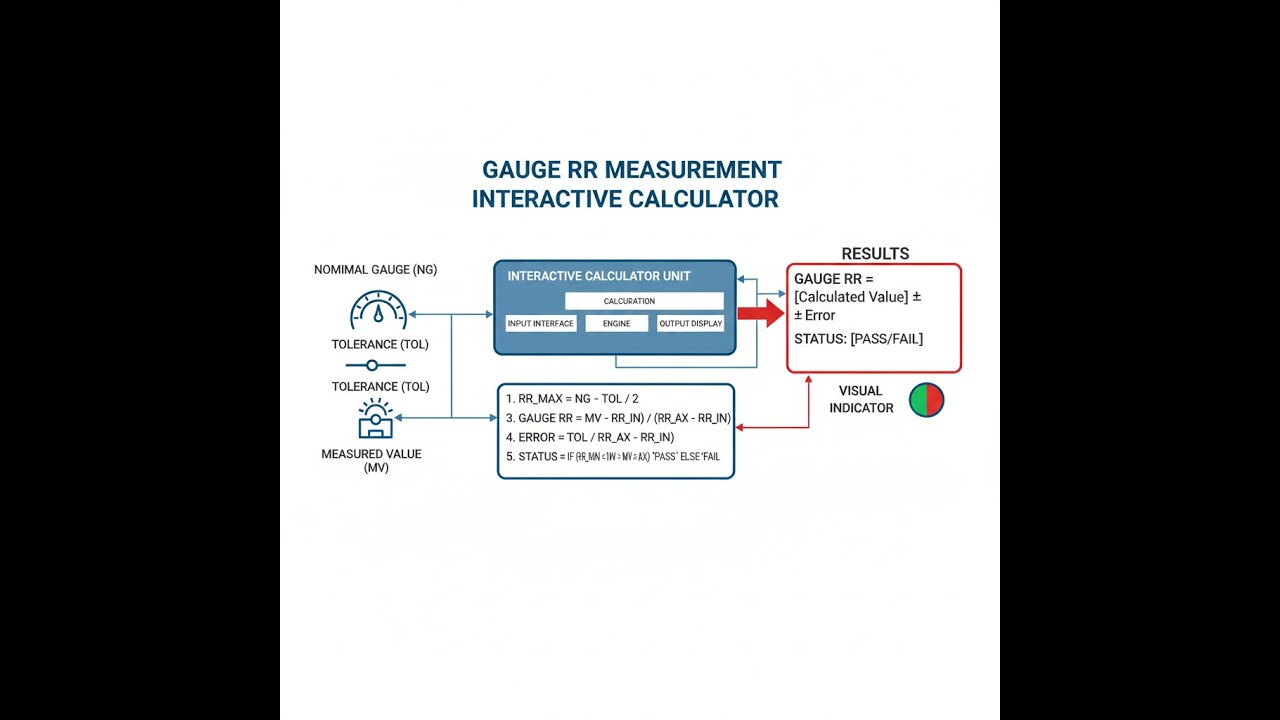
Visual Diagram

Gauge R&R Interactive Calculator
How to Use This Calculator
- Select your Calculation Mode — Standard, ANOVA, Percent Tolerance, NDC, or Acceptance Criteria.
- Enter your Equipment Variation (EV), Appraiser Variation (AV), Part Variation (PV), and Specification Tolerance — or, if using ANOVA mode, enter Range Average, number of Trials, Operators, Parts, and Range of Part Averages.
- Check that all values are positive and match the units of your measurement study.
- Click Calculate to see your result.
gauge r&r measurement interactive visualizer
See how equipment variation (EV) and appraiser variation (AV) combine to create total gauge R&R, and understand when your measurement system is trustworthy versus when it's masking real part variation. Adjust the variation sources to see immediate impact on %GRR acceptance criteria.
GAUGE R&R
0.025
%GRR
38.5%
TOTAL VAR
0.065
STATUS
POOR
FIRGELLI Automations — Interactive Engineering Calculators
Gauge R&R Equations
Use the formula below to calculate Gauge R&R (GRR).
Gauge R&R (GRR) Calculation
GRR = √(EV² + AV²)
Where:
GRR = Gauge Repeatability and Reproducibility
EV = Equipment Variation (repeatability)
AV = Appraiser Variation (reproducibility)
Use the formula below to calculate Total Variation (TV).
Total Variation (TV)
TV = √(GRR² + PV²)
Where:
TV = Total Variation
PV = Part Variation (part-to-part variation)
Use the formula below to calculate Percent GRR of Total Variation.
Percent GRR of Total Variation
%GRR = (GRR / TV) × 100%
Acceptance Criteria:
%GRR less than 10% = Acceptable
%GRR 10-30% = Marginal (may be acceptable)
%GRR greater than 30% = Unacceptable
Use the formula below to calculate Percent of Tolerance.
Percent of Tolerance
%Tolerance = (6 × GRR / Tolerance) × 100%
Where:
Tolerance = Upper Specification Limit minus Lower Specification Limit
The factor 6 represents ±3 standard deviations (99.73% coverage)
Use the formula below to calculate Number of Distinct Categories (NDC).
Number of Distinct Categories (NDC)
NDC = ⌊1.41 × (PV / GRR)⌋
Where:
⌊ ⌋ = Floor function (round down to nearest integer)
NDC ≥ 5 is generally required for adequate discrimination
The factor 1.41 is √2, accounting for measurement system resolution
Use the formula below to calculate Equipment Variation using the ANOVA method.
ANOVA Method - Equipment Variation
EV = (R̄ / d2) × K1
Where:
R̄ = Average range across all operators and trials
d2 = Control chart constant (depends on number of trials)
K1 = Study variation constant (typically 5.15 for 99% confidence)
Simple Example
Given: EV = 0.010, AV = 0.010, PV = 0.050, Specification Tolerance = 0.200
GRR = √(0.010² + 0.010²) = √(0.0002) ≈ 0.0141
TV = √(0.0141² + 0.050²) ≈ 0.0519
%GRR = (0.0141 / 0.0519) × 100% ≈ 27.2% — marginal system, investigate before relying on it for final inspection.
NDC = ⌊1.41 × (0.050 / 0.0141)⌋ = ⌊5.0⌋ = 5 — barely adequate discrimination.
Theory & Engineering Applications
Fundamental Principles of Measurement System Analysis
Gauge Repeatability and Reproducibility (Gauge R&R) studies form the cornerstone of measurement system analysis in modern manufacturing and quality control. The methodology quantifies two distinct sources of measurement error: repeatability represents the inherent variation of the measurement equipment itself when measuring the same part multiple times under identical conditions, while reproducibility captures the variation introduced by different operators using the same equipment. This distinction is crucial because it allows engineers to identify whether measurement problems stem from equipment calibration issues or operator training deficiencies.
The statistical foundation of Gauge R&R relies on variance decomposition, where total observed variation is partitioned into measurement system variation and actual part-to-part variation. The critical insight that many practitioners miss is that a measurement system doesn't need to be perfect—it only needs to be precise enough to detect meaningful variation in the parts being measured. A common misconception is that any detectable measurement variation is problematic, but in reality, measurement systems consuming less than 10% of the total variation budget still leave 90% of observed variation attributable to actual part differences, which is sufficient for most process control applications.
The acceptance criterion of less than 10% GRR for acceptable systems, 10-30% for marginal systems, and greater than 30% for unacceptable systems emerged from decades of industrial practice across automotive, aerospace, and electronics manufacturing. These thresholds represent practical compromises between measurement accuracy and economic feasibility. However, a non-obvious limitation is that these criteria assume the part variation in the study is representative of production variation—if the study parts are carefully selected to span the full specification range, the calculated %GRR may be artificially low. Conversely, if study parts cluster near the nominal dimension, %GRR will appear inflated even for capable measurement systems.
ANOVA Method vs. Range Method
Two primary calculation methods exist for Gauge R&R studies: the Average and Range (X̄-R) method and the Analysis of Variance (ANOVA) method. The X̄-R method, being computationally simpler, uses range statistics and control chart constants (d₂ values) to estimate variation components. This method is adequate for most applications and forms the basis of many production floor studies because it can be performed with basic spreadsheet tools and doesn't require advanced statistical software.
The ANOVA method provides more detailed information by calculating operator-by-part interaction effects, which reveal whether certain operators consistently measure certain parts differently than others. This interaction term often indicates that parts have features that are difficult to measure consistently, such as surface finish variations, measurement location ambiguity, or fixturing problems. In precision manufacturing environments like medical device production or semiconductor fabrication, the ANOVA method's additional insight justifies its computational complexity. The interaction variance, when significant, must be included in the reproducibility calculation, potentially pushing an apparently acceptable measurement system into the marginal or unacceptable range.
Number of Distinct Categories and Resolution
The Number of Distinct Categories (NDC) metric provides a practical interpretation of measurement system capability that transcends percentage calculations. NDC answers the question: "How many statistically distinct groups can this measurement system reliably place parts into?" For continuous process control, the rule of thumb requires NDC ≥ 5, meaning the system can distinguish at least five quality levels. This ensures sufficient resolution for process improvement efforts where detecting subtle shifts in the process mean is critical.
An often-overlooked aspect of NDC is its relationship to gage resolution. Digital measurement equipment displaying to more decimal places doesn't automatically improve NDC if the underlying sensor noise hasn't decreased proportionally. A caliper reading to 0.0001 inches with poor repeatability may have lower effective discrimination than a properly calibrated indicator reading to 0.001 inches. This principle becomes critical when specifying measurement equipment—purchasing higher-resolution instruments without addressing fundamental repeatability issues wastes resources without improving measurement capability.
Worked Example: Shaft Diameter Measurement System
Consider a manufacturing facility producing precision shafts for automotive transmissions. The nominal diameter is 25.000 mm with a tolerance of ±0.050 mm (total tolerance = 0.100 mm). Three operators each measure ten parts three times using a bench-mounted digital indicator. The following data represents calculated variation components from the study:
Given Data:
- Equipment Variation (EV) = 0.0087 mm
- Appraiser Variation (AV) = 0.0065 mm
- Part Variation (PV) = 0.0423 mm
- Specification Tolerance = 0.100 mm
Step 1: Calculate Gauge R&R (GRR)
GRR = √(EV² + AV²) = √(0.0087² + 0.0065²) = √(0.00007569 + 0.00004225) = √0.00011794 = 0.01086 mm
Step 2: Calculate Total Variation (TV)
TV = √(GRR² + PV²) = √(0.01086² + 0.0423²) = √(0.0001180 + 0.001789) = √0.001907 = 0.04367 mm
Step 3: Calculate %GRR of Total Variation
%GRR = (GRR / TV) × 100% = (0.01086 / 0.04367) × 100% = 24.87%
Step 4: Calculate Individual Component Percentages
%EV = (EV / TV) × 100% = (0.0087 / 0.04367) × 100% = 19.92%
%AV = (AV / TV) × 100% = (0.0065 / 0.04367) × 100% = 14.89%
%PV = (PV / TV) × 100% = (0.0423 / 0.04367) × 100% = 96.88%
Note that these percentages don't sum to 100% because they're based on standard deviations, not variances. To verify: √(19.92² + 14.89²) = 24.88%, confirming our GRR calculation.
Step 5: Calculate %Tolerance
%Tolerance = (6 × GRR / Tolerance) × 100% = (6 × 0.01086 / 0.100) × 100% = (0.06516 / 0.100) × 100% = 65.16%
Step 6: Calculate Number of Distinct Categories (NDC)
NDC = ⌊1.41 × (PV / GRR)⌋ = ⌊1.41 × (0.0423 / 0.01086)⌋ = ⌊1.41 × 3.894⌋ = ⌊5.491⌋ = 5
Interpretation: This measurement system falls into the marginal category with %GRR = 24.87%, which is between 10% and 30%. The NDC of 5 indicates adequate discrimination capability for distinguishing between different part populations. The dominant component of GRR is equipment variation (19.92%) rather than appraiser variation (14.89%), suggesting that calibration or equipment upgrade would be more beneficial than additional operator training. The %Tolerance value of 65.16% indicates the measurement system consumes a significant portion of the specification tolerance, meaning process capability studies using this gage will underestimate true process capability by attributing measurement error to process variation.
Recommended Actions: Given the marginal result, the team should evaluate whether this measurement system adequacy is acceptable for the application. For in-process control where trend detection matters more than absolute accuracy, this system may be sufficient. However, for final inspection or Cpk calculations, improving the measurement system—perhaps by using a coordinate measuring machine (CMM) for critical dimensions—would provide more reliable quality data. The fact that equipment variation dominates suggests investigating indicator mounting rigidity, part clamping consistency, and potential temperature effects on the measurement setup.
Application Across Industries
In pharmaceutical manufacturing, Gauge R&R studies validate analytical methods for active pharmaceutical ingredient (API) concentration measurement. Here, %GRR criteria may be tightened to less than 5% because regulatory compliance depends on measurement accuracy. Laboratory equipment like HPLC systems undergo rigorous R&R studies where analyst-to-analyst variation (reproducibility) often exceeds equipment variation due to subtle differences in sample preparation techniques.
Aerospace manufacturers conducting Gauge R&R on coordinate measuring machines (CMMs) face unique challenges because complex geometric dimensioning and tolerancing (GD&T) characteristics introduce additional variation sources. Profile tolerance measurements, for example, involve software algorithms that can contribute to apparent reproducibility differences when different operators use different datum establishment strategies, even on the same CMM using identical fixturing.
Electronics assembly operations use Gauge R&R for solder joint inspection systems, both automated optical inspection (AOI) and manual visual inspection. These studies reveal that human visual inspection typically shows higher reproducibility variation than repeatability variation—different inspectors applying different acceptance standards for borderline conditions. This finding drives investment in automated systems where repeatability dominates and can be controlled through calibration, producing more consistent accept/reject decisions across production shifts.
Practical Applications
Scenario: Quality Manager Validating New CMM Investment
Jennifer is a quality manager at a precision machining company that just installed a $175,000 coordinate measuring machine (CMM) to replace older manual measurement equipment. Before releasing the CMM for production inspection, she conducts a comprehensive Gauge R&R study with three trained operators measuring 10 representative parts three times each. Using the ANOVA method calculator, she determines that Equipment Variation is 0.0034 mm, Appraiser Variation is 0.0019 mm, and Part Variation is 0.0521 mm across the critical feature dimensions. The calculator shows %GRR of 7.5% and NDC of 13, both excellent results that validate the CMM for production use. Jennifer's study documentation becomes part of the quality management system, satisfying ISO 9001 requirements and providing objective evidence that the measurement system is suitable for verifying conformance to customer specifications. The low appraiser variation component confirms that operator training was effective, while the dominant part variation indicates the system successfully detects actual manufacturing differences.
Scenario: Manufacturing Engineer Troubleshooting High Scrap Rates
Carlos, a manufacturing engineer at an injection molding facility, is investigating why scrap rates increased from 2% to 8% after implementing tighter wall thickness tolerances on medical device housings. Suspecting the measurement system rather than the process itself, he performs a Gauge R&R study on the ultrasonic thickness gage used for 100% inspection. The calculator reveals %GRR of 34%, clearly in the unacceptable range, with equipment variation being the dominant component at 29% of total variation. This finding explains the scrap rate problem—parts near the specification limits are being incorrectly accepted or rejected based on measurement noise rather than actual dimensions. Carlos discovers the ultrasonic gage transducer has degraded over time and the calibration block doesn't span the measurement range adequately. After replacing the transducer and conducting proper calibration with traceable standards, a follow-up study shows %GRR dropping to 12% (marginal but acceptable for this application), and production scrap rates return to 2.5%. The economic impact is immediate: preventing approximately $45,000 per month in unnecessary scrap costs, easily justifying the $3,800 spent on the new transducer and calibration service.
Scenario: Six Sigma Black Belt Preparing for DMAIC Project
Marcus, a Six Sigma Black Belt at an automotive tier-one supplier, is launching a DMAIC project to improve the capability (Cpk) of a bearing housing machining process currently running at Cpk = 0.87, below the customer requirement of 1.33. Before beginning his process improvement work, he conducts Gauge R&R studies on all measurement systems used to evaluate the critical-to-quality characteristics. For the bore diameter measurement using a three-point bore gage, the calculator shows %GRR of 18% (marginal) with NDC of 4. This finding is crucial—the measurement system cannot adequately distinguish between parts, meaning the reported Cpk of 0.87 is artificially deflated by measurement error. Marcus calculates that if the measurement system were perfect, the true process Cpk would be approximately 1.05, still below target but significantly better than the apparent 0.87. He now has two improvement paths: upgrade the measurement system to an air gage with better repeatability (reducing %GRR to less than 10%), or improve the machining process itself. His economic analysis shows that a $12,000 air gage investment combined with modest process improvements will achieve the target Cpk, whereas process improvements alone would require approximately $60,000 in new tooling and fixtures—the Gauge R&R study fundamentally changed his project strategy and saved substantial capital expenditure.
Frequently Asked Questions
Free Engineering Calculators
Explore our complete library of free engineering and physics calculators.
Browse All Calculators →🔗 Explore More Free Engineering Calculators
About the Author
Robbie Dickson — Chief Engineer & Founder, FIRGELLI Automations
Robbie Dickson brings over two decades of engineering expertise to FIRGELLI Automations. With a distinguished career at Rolls-Royce, BMW, and Ford, he has deep expertise in mechanical systems, actuator technology, and precision engineering.
Need to implement these calculations?
Explore the precision-engineered motion control solutions used by top engineers.


