Availability Mtbf Interactive Calculator

The Availability MTBF Calculator is an essential tool for reliability engineers, maintenance managers, and operations professionals who need to quantify system uptime, predict failure intervals, and optimize maintenance schedules. This calculator computes key reliability metrics including system availability, Mean Time Between Failures (MTBF), Mean Time To Repair (MTTR), and failure rates, enabling data-driven decisions about equipment reliability, spare parts inventory, and maintenance resource allocation across manufacturing, aerospace, utilities, and critical infrastructure sectors.

📐 Browse all free engineering calculators

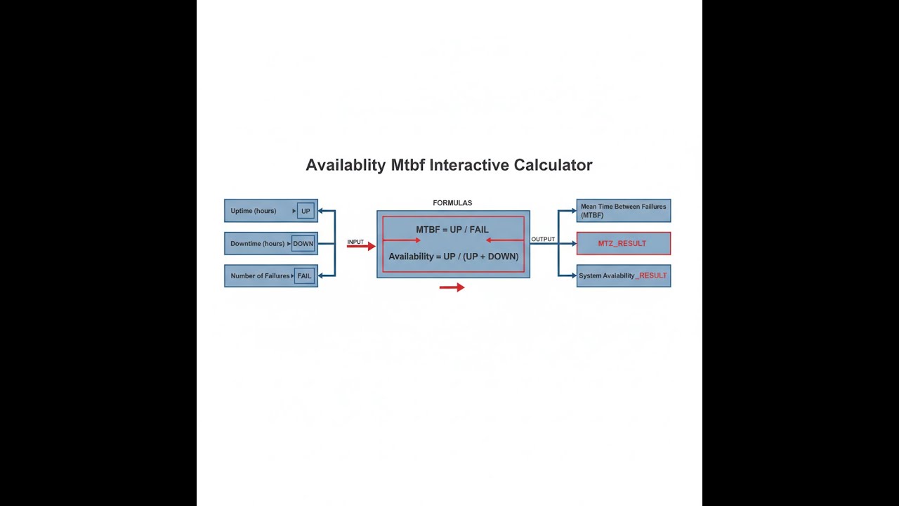
System Reliability Diagram

Availability & MTBF Calculator

Reliability Equations

Theory & Engineering Applications

System availability and Mean Time Between Failures represent fundamental metrics in reliability engineering, quantifying the fraction of time a system or component performs its intended function. These parameters drive critical business decisions including maintenance strategy selection, spare parts inventory optimization, warranty cost estimation, and capital equipment procurement. Understanding the mathematical relationships between availability, MTBF, MTTR, and failure rates enables engineers to design systems that meet operational requirements while balancing reliability investment against total cost of ownership.

Fundamental Reliability Theory

Availability is defined as the probability that a system is operational at any given point in time, expressed as the ratio of uptime to total time. The relationship A = MTBF/(MTBF + MTTR) emerges from renewal theory, assuming failures follow a stationary stochastic process where the system alternates between operational and repair states. This formulation applies to repairable systems where components are restored to functionality after failure, distinguishing it from reliability R(t) = e^-λt which describes non-repairable systems or time-to-first-failure scenarios.

The assumption of exponential failure distribution (constant hazard rate λ = 1/MTBF) simplifies analysis but has important limitations. Real-world systems often exhibit bathtub curves with decreasing hazard rates during burn-in, constant rates during useful life, and increasing rates during wear-out. The exponential model provides conservative estimates during the constant hazard phase but becomes inaccurate for aging equipment. Weibull distributions with shape parameter β ≠ 1 more accurately model wear-out (β greater than 1) and infant mortality (β less than 1), requiring modified MTBF calculations incorporating the gamma function: MTBF = η·Γ(1 + 1/β) where η is the Weibull scale parameter.

MTTR Components and Hidden Losses

Mean Time To Repair encompasses more than wrench time—it includes failure detection lag, diagnostic time, spare parts procurement and logistics, administrative delays, and system restart/testing. In practice, MTTR often exceeds active repair time by factors of 2-5×. A hydraulic pump mechanical seal replacement might require 3 hours of actual work, but if failure detection takes 45 minutes, diagnosis takes 1 hour, parts ordering requires overnight shipping, and post-repair testing takes 2 hours, the effective MTTR becomes 27 hours. This distinction between Mean Time To Repair (hands-on work) and Mean Time To Restore (total downtime) significantly impacts availability calculations.

Condition-based monitoring systems reduce MTTR by enabling predictive maintenance before failures occur, eliminating detection lag and reducing unplanned downtime. Vibration analysis on rotating equipment can identify bearing degradation weeks before failure, allowing planned replacement during scheduled maintenance windows rather than emergency repairs. This shifts maintenance from reactive (high MTTR) to proactive (lower effective MTTR through planned downtime), improving availability without necessarily changing MTBF.

Series and Parallel System Configurations

For systems with multiple components in series (where all must function), overall availability equals the product of individual availabilities: A_system = A₁ × A₂ × ... × A_n. A production line with six stations each having 98% availability achieves only A_system = 0.98⁶ = 88.6% overall availability, demonstrating how serial dependencies rapidly degrade system performance. This multiplicative effect explains why complex systems with many components require extremely high individual component reliability to achieve acceptable system-level availability.

Parallel redundancy (where only one component needs to function) dramatically improves availability through the complement rule: A_parallel = 1 - (1 - A₁)(1 - A₂)...(1 - A_n). Two pumps in hot standby configuration, each with 95% availability, achieve system availability of 1 - (1 - 0.95)² = 99.75%. However, common-mode failures (events affecting both redundant components simultaneously, such as contaminated fuel or electrical surges) reduce practical availability below theoretical calculations. A common-mode failure rate of 5% reduces the dual-pump availability from 99.75% to approximately 99.5%, illustrating the importance of failure independence assumptions.

Industry-Specific Availability Requirements

Different industries impose dramatically different availability targets based on economic consequences of downtime and safety criticality. Data center Tier IV facilities require 99.995% availability (26 minutes annual downtime), achieved through N+1 redundancy on all systems including cooling, power, and network infrastructure. Telecommunications carriers target "five nines" (99.999%) or 5.26 minutes annual downtime for critical switching equipment, driving mean time to repair below 15 minutes through extensive sparing and trained on-site personnel.

Manufacturing availability requirements depend on production value streams and buffering capacity. High-volume automotive assembly lines with minimal work-in-process buffers require 95-98% availability for critical bottleneck operations, translating to MTBF values of 400-800 hours with 4-hour MTTR targets. Conversely, batch chemical processes with days of in-process inventory can tolerate 85-90% availability on secondary equipment. Mining operations often design for 85-90% availability on mobile equipment, accounting for harsh operating conditions and remote locations that increase MTTR through longer parts delivery times.

Availability vs. Utilization Distinction

A critical but often misunderstood concept: availability measures technical uptime (ready to operate), while utilization measures productive output (actually operating). A machine can have 99% availability but 60% utilization if production scheduling, material shortages, or labor constraints leave it idle 40% of available time. Overall Equipment Effectiveness (OEE) combines availability with performance efficiency and quality rate: OEE = Availability × Performance × Quality. A stamping press with 95% availability, 85% speed efficiency (due to intentional slowdowns), and 98% first-pass yield achieves OEE = 0.95 × 0.85 × 0.98 = 79.1%, revealing significant improvement opportunities despite apparently high availability.

Worked Example: Production Line Availability Analysis

Consider a semiconductor wafer fabrication tool used for photolithography in a 24/7 fab. Over one quarter (2190 hours), the equipment experiences the following:

• Number of failures: 14 unplanned stops
• Total downtime: 127 hours (including all detection, diagnosis, repair, and restart time)
• Total uptime: 2063 hours
• Preventive maintenance: 3 scheduled events consuming 18 hours (counted as uptime for availability purposes)

Step 1: Calculate actual availability from uptime/downtime

A = T_uptime / (T_uptime + T_downtime) = 2063 / (2063 + 127) = 2063 / 2190 = 0.9420 = 94.20%

Step 2: Calculate MTBF from operational data

MTBF = T_total / N_failures = 2190 / 14 = 156.43 hours between failures

Step 3: Calculate MTTR from downtime and failure count

MTTR = T_downtime / N_failures = 127 / 14 = 9.07 hours per repair event

Step 4: Verify availability using MTBF/MTTR formula

A = MTBF / (MTBF + MTTR) = 156.43 / (156.43 + 9.07) = 156.43 / 165.50 = 0.9452 = 94.52%

The slight discrepancy (94.20% vs 94.52%) arises because the MTBF/MTTR formula assumes steady-state conditions while the direct calculation reflects the actual measurement period. The tool's current performance falls short of the fab's 96% availability target.

Step 5: Determine required MTTR to achieve 96% availability target

Rearranging A = MTBF / (MTBF + MTTR) to solve for MTTR:

MTTR = MTBF × (1 - A) / A = 156.43 × (1 - 0.96) / 0.96 = 156.43 × 0.04 / 0.96 = 6.52 hours

To reach 96% availability with current MTBF = 156.43 hours, MTTR must be reduced from 9.07 hours to 6.52 hours—a 28% reduction requiring approximately 2.5 hours per event improvement.

Step 6: Alternative approach—improve MTBF while holding MTTR constant

MTBF = (MTTR × A) / (1 - A) = (9.07 × 0.96) / (1 - 0.96) = 8.71 / 0.04 = 217.75 hours

Alternatively, maintaining MTTR = 9.07 hours requires increasing MTBF from 156.43 to 217.75 hours—a 39% improvement through better preventive maintenance, higher quality spare parts, or improved operating procedures.

Step 7: Calculate failure rate and interpret

λ = 1 / MTBF = 1 / 156.43 = 0.006392 failures per hour = 0.6392% per hour

This translates to approximately 56 failures per year (8760 hours), significantly higher than the "world-class" semiconductor fab target of 24-30 failures per tool per year, suggesting systematic reliability improvement initiatives are warranted.

This example illustrates the practical decision framework: reliability teams can improve availability by increasing MTBF (redesign, better parts, preventive maintenance), decreasing MTTR (spare parts stocking, technician training, diagnostic tools), or both. The economic optimization balances improvement costs against downtime costs, typically finding MTTR reduction more cost-effective initially (diminishing returns beyond certain thresholds), then pursuing MTBF improvements for further gains.

For additional reliability engineering resources and calculation tools, visit the FIRGELLI Engineering Calculator Library featuring specialized calculators for maintenance optimization, reliability prediction, and system availability analysis.

Practical Applications

Frequently Asked Questions