Designing a retaining wall, sheet pile, or basement wall means getting the lateral earth pressure right — underestimate it and the structure fails, overestimate it and you waste material. Use this Active Earth Pressure Rankine Calculator to calculate pressure distribution, resultant force, and overturning moments using wall height, soil unit weight, friction angle, cohesion, and surcharge load. It's essential for foundation engineering, coastal structures, and underground construction. This page includes the full Rankine formula, a worked example, engineering theory, and a detailed FAQ.
What is Active Earth Pressure?
Active earth pressure is the lateral force that soil exerts on a retaining structure when the wall moves slightly away from the backfill. It represents the minimum stable pressure the soil can apply — the force you must design against to keep a retaining wall standing.
Simple Explanation
Think of soil like a stack of books leaning against a bookend. If the bookend tilts outward even slightly, the books push against it with a predictable force — that's active earth pressure. The looser or heavier the soil, the harder it pushes. Rankine's theory gives you a straightforward formula to calculate exactly how hard, so you can size the wall to hold it.
📐 Browse all 1000+ Interactive Calculators
Table of Contents
Retaining Wall Diagram

Active Earth Pressure Rankine Calculator
How to Use This Calculator
- Select a calculation mode from the dropdown — choose what you want to solve for (pressure distribution, resultant force, overturning moment, Ka coefficient, wall height, or soil density).
- Enter the known values: wall height (m), soil unit weight (kN/m³), friction angle (degrees), cohesion (kPa), and surcharge load (kPa) as applicable to your selected mode.
- Check that all inputs are physically valid — friction angle must be between 0° and 90°, all weights and heights must be positive.
- Click Calculate to see your result.
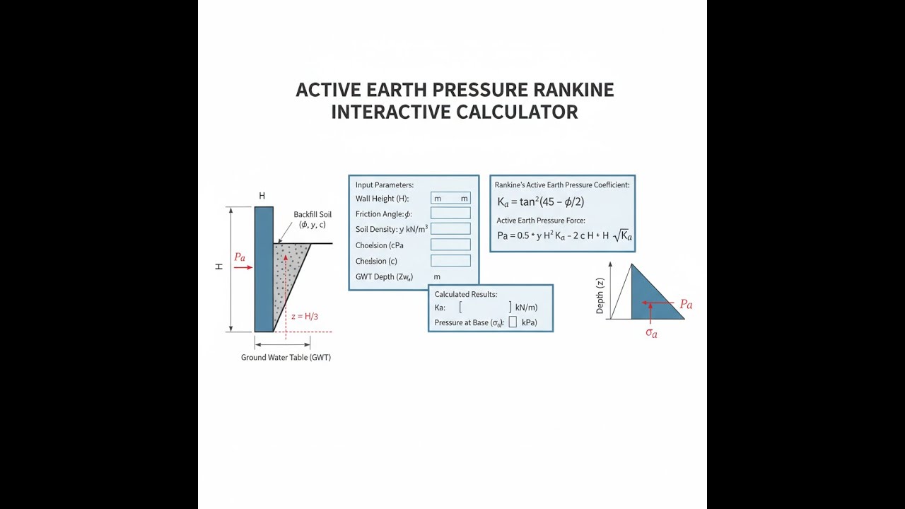
Active Earth Pressure Rankine Interactive Calculator
Visualize lateral earth pressure distribution on retaining walls using Rankine theory. Adjust soil properties and wall height to see how pressure varies with depth and understand the critical forces your structure must resist.
Ka COEFFICIENT
0.333
MAX PRESSURE
24.0 kPa
RESULTANT FORCE
48.0 kN/m
MOMENT ARM
1.33 m
FIRGELLI Automations — Interactive Engineering Calculators
Equations & Formulas
Use the formula below to calculate the active earth pressure coefficient.
Active Earth Pressure Coefficient (Rankine):
Ka = tan²(45° - φ/2)
Lateral Earth Pressure at Depth z:
σa = Ka(γz + q) - 2c√Ka
Resultant Active Force (per unit width):
Pa = ½KaγH² + KaqH - 2c√KaH
Location of Resultant Force (from base):
z̄ = H/3 × (2σbottom + σtop) / (σbottom + σtop)
Overturning Moment about Base:
M = Pa × z̄
Where:
- Ka = Active earth pressure coefficient (dimensionless)
- φ = Internal friction angle of soil (degrees)
- σa = Active lateral earth pressure at depth z (kPa)
- γ = Unit weight of soil (kN/m³)
- z = Depth below ground surface (m)
- H = Total height of retaining wall (m)
- q = Uniform surcharge load at surface (kPa)
- c = Soil cohesion (kPa)
- Pa = Total active force per unit width of wall (kN/m)
- z̄ = Height of resultant force location above base (m)
- M = Overturning moment about wall base (kN·m/m)
Simple Example
A 4 m retaining wall backs a dry cohesionless sand (γ = 18 kN/m³, φ = 30°, c = 0, no surcharge).
- Ka = tan²(45° − 15°) = tan²(30°) = 0.333
- Pressure at base: σₐ = 0.333 × 18 × 4 = 24.0 kPa
- Resultant force: Pₐ = ½ × 0.333 × 18 × 4² = 48.0 kN/m, acting 1.33 m above the base
Theory & Engineering Applications
Rankine's active earth pressure theory, developed by William Rankine in 1857, remains one of the most widely applied classical methods in geotechnical engineering for predicting lateral earth pressures on retaining structures. The theory establishes the minimum lateral pressure that develops when a soil mass is allowed to expand horizontally until reaching a state of plastic equilibrium, characterized by the formation of a failure plane at 45° + φ/2 from the horizontal.
Fundamental Assumptions and Limitations
Rankine's method operates under several critical assumptions that define its applicability boundaries. The theory assumes a semi-infinite soil mass with a vertical back face, homogeneous soil properties, and a horizontal or uniformly sloping backfill surface. The soil must be in a state of plastic equilibrium, meaning sufficient wall movement has occurred to mobilize the full shear strength of the soil along failure planes. For typical granular soils, this displacement ranges from 0.001H to 0.004H, where H represents wall height—meaning a 5-meter wall requires only 5 to 20 millimeters of outward movement to achieve active conditions.
A critical but often overlooked limitation involves the assumption of a smooth wall-soil interface with zero wall friction. Real retaining structures develop interface friction that reduces lateral pressures below Rankine predictions, making the method inherently conservative. The Coulomb theory accounts for wall friction explicitly, but Rankine's simplicity and mathematical elegance make it preferred for preliminary design, especially when wall friction angles are uncertain or when conservative estimates provide additional safety margins.
Active Earth Pressure Coefficient Derivation
The active earth pressure coefficient Ka emerges from Mohr's circle analysis of stress states at failure. In the active condition, the major principal stress acts vertically (from soil self-weight), while the minor principal stress acts horizontally (lateral pressure on the wall). At the failure condition, the Mohr's circle becomes tangent to the Mohr-Coulomb failure envelope, establishing a geometric relationship between principal stresses and soil strength parameters. For cohesionless soils, this relationship simplifies to Ka = tan²(45° - φ/2), revealing an inverse exponential relationship with friction angle.
This mathematical form has profound practical implications. A soil with φ = 30° yields Ka = 0.333, meaning lateral pressures are one-third of vertical pressures. Increasing friction angle to 35° reduces Ka to 0.271—a 19% reduction in lateral force from just a 5-degree strength increase. This sensitivity underscores why accurate friction angle determination through triaxial or direct shear testing is critical for economical retaining wall design. Conversely, it also explains why contractors sometimes encounter wall failures when actual soil strengths are lower than assumed design values, particularly in saturated or poorly compacted conditions.
Cohesion Effects and Tension Zone Formation
The presence of cohesion introduces a subtractive term (2c√Ka) that reduces lateral pressures throughout the soil profile. For purely cohesive soils (φ = 0), this reduction can theoretically produce negative (tensile) pressures in the upper portion of the wall. Since soils cannot sustain significant tension, a tension crack forms that extends to a depth where lateral pressure reaches zero. This depth z₀ = 2c/(γ√Ka) defines the tension zone boundary, which must be considered in design to avoid overestimating resistance.
In partially saturated clay soils with typical cohesion values of 10-30 kPa, tension cracks can extend 1.5 to 3.5 meters deep—a substantial portion of many retaining walls. These cracks often fill with water during rainfall events, creating hydrostatic pressure that adds significant lateral load not accounted for in dry soil calculations. This mechanism has contributed to numerous retaining wall failures in clayey soils, particularly in regions with seasonal precipitation. Modern practice often conservatively neglects cohesion in active pressure calculations for permanent structures, treating it as a safety factor rather than a reliable strength component.
Applications Across Engineering Disciplines
Basement wall design for commercial and residential buildings represents one of the most common applications of Rankine theory. Structural engineers use active pressure calculations to determine required wall thickness, reinforcement spacing, and lateral bracing requirements for concrete or masonry basement walls. For a typical 3-meter basement with dense sandy backfill (γ = 19 kN/m³, φ = 35°), the calculator shows a resultant force of approximately 46 kN/m acting 1 meter above the base, requiring foundation designs that resist both overturning moments and sliding forces.
Coastal and marine engineering extensively employs Rankine calculations for seawall and bulkhead design. Tidal structures experience both submerged soil pressures (using buoyant unit weight γ' = γ - 9.81 kN/m³) and hydrostatic water pressure. The combined loading often governs structural dimensions and pile penetration depths. Sheet pile walls driven into saturated sand with φ = 32° and submerged unit weight of 10 kN/m³ experience approximately 70% less active earth pressure than identical dry conditions—a critical distinction for economical marine structure design.
Mining and excavation support systems rely on active pressure theory to design temporary shoring and permanent slope stabilization. Open-pit mines cutting through overburden layers use Rankine-based calculations to determine required setback distances and the necessity of toe berms or bench systems to maintain stable slopes. Deep basement excavations in urban environments utilize sequential bracing systems designed using active pressure distributions to support sheet piling or diaphragm walls during staged excavation.
Worked Example: Basement Retaining Wall Design
Consider the design of a basement retaining wall for a commercial building with the following site conditions:
- Wall height H = 4.2 meters
- Backfill soil: medium dense sand, γ = 18.5 kN/m³
- Internal friction angle φ = 32° (from triaxial testing)
- Cohesion c = 0 kPa (conservative for granular soil)
- Surface surcharge q = 12 kPa (equivalent to light vehicle loading)
Step 1: Calculate Active Earth Pressure Coefficient
Ka = tan²(45° - φ/2) = tan²(45° - 32°/2) = tan²(29°) = (0.5543)² = 0.3073
Step 2: Determine Pressure Distribution
At the top surface (z = 0):
σₐ(top) = Ka × q - 2c√Ka = 0.3073 × 12 - 0 = 3.69 kPa
At the base (z = H = 4.2 m):
σₐ(bottom) = Ka(γH + q) - 2c√Ka = 0.3073(18.5 × 4.2 + 12) - 0
σₐ(bottom) = 0.3073(77.7 + 12) = 0.3073 × 89.7 = 27.56 kPa
Step 3: Calculate Resultant Active Force
The pressure distribution forms a trapezoid. The resultant force per meter of wall length is:
Pₐ = ½(σₐ(top) + σₐ(bottom)) × H = ½(3.69 + 27.56) × 4.2 = ½ × 31.25 × 4.2 = 65.63 kN/m
Step 4: Determine Force Location
For a trapezoidal distribution, the resultant acts at:
z̄ = H/3 × (2σₐ(bottom) + σₐ(top))/(σₐ(bottom) + σₐ(top))
z̄ = 4.2/3 × (2 × 27.56 + 3.69)/(27.56 + 3.69) = 1.4 × 58.81/31.25 = 1.4 × 1.882 = 2.63 meters from base
Note: This is significantly higher than the H/3 = 1.4 m location for a purely triangular distribution (no surcharge), demonstrating how surface loads elevate the resultant force location.
Step 5: Calculate Overturning Moment
M = Pₐ × z̄ = 65.63 × 2.63 = 172.6 kN·m per meter of wall length
Step 6: Design Implications
For a concrete cantilever retaining wall with a 0.4-meter thick stem, the required base width must resist both overturning and sliding. Assuming a concrete density of 24 kN/m³ and a 3-meter base width, the resisting moment from the wall's self-weight alone is approximately 240 kN·m/m. The factor of safety against overturning is 240/172.6 = 1.39, which is below the typical required minimum of 2.0. This calculation immediately indicates that either the base must be widened to 4+ meters, or the backfill soil quality must be improved through compaction to achieve higher friction angles, or a soil reinforcement system (geogrids) must be incorporated to reduce lateral pressures.
This worked example demonstrates how Rankine calculations directly inform structural sizing decisions and cost implications. A 33% increase in base width (from 3m to 4m) represents substantial additional concrete volume and foundation excavation costs, making soil investigation accuracy and backfill quality control economically significant factors beyond their safety implications.
Integration with Modern Design Codes
Contemporary design standards including AASHTO LRFD Bridge Design Specifications and Eurocode 7 incorporate Rankine-based active pressure calculations within load and resistance factor design (LRFD) frameworks. These codes apply partial factors to both soil strength parameters and resulting forces to achieve target reliability indices. Typical LRFD approaches reduce friction angles by 3-5 degrees (or multiply Ka by 1.2-1.5) while increasing resultant forces by 1.5-1.75 to account for material variability and model uncertainty. Explore additional calculation tools at the engineering calculators hub for related geotechnical and structural analysis methods.
The interaction between active pressure theory and modern performance-based design has led to sophisticated numerical modeling approaches using finite element analysis to validate Rankine predictions for complex geometries. However, these advanced methods invariably begin with Rankine calculations as baseline values to verify numerical model convergence and ensure results fall within physically reasonable bounds. This enduring role, 165 years after its publication, testifies to the theory's fundamental soundness and practical utility in engineering practice.
Practical Applications
Scenario: Residential Basement Waterproofing Design
Marcus, a structural engineer with a regional design firm, is preparing construction documents for a luxury home featuring a full 3.6-meter-deep basement in an area with medium-dense sandy soil. The architect has specified exterior waterproofing and landscaping that will place 0.6 meters of topsoil and plantings adjacent to the basement wall, creating an additional surcharge. Using this calculator with the site's soil parameters (γ = 17.8 kN/m³, φ = 31° from boring logs, 8 kPa surcharge from planned landscaping), Marcus calculates an active earth pressure distribution ranging from 2.4 kPa at the top to 22.7 kPa at the footing level. The resultant force of 45.2 kN/m acting 1.26 meters above the base informs his decision to specify 250mm concrete wall thickness with #5 rebar at 300mm spacing, ensuring adequate moment capacity while maintaining economical material usage. The calculation also alerts him that the overturning moment of 57 kN·m/m requires a minimum 2.8-meter-wide footing to achieve the 2.5 factor of safety against overturning specified in the local building code. This systematic approach prevents the common design error of underestimating surcharge effects, which has led to numerous basement wall cracking failures in similar residential projects.
Scenario: Highway Retaining Wall Cost Optimization
Jennifer, a geotechnical consultant for a state transportation department, is evaluating value engineering alternatives for a 6.5-meter highway retaining wall project originally designed with expensive mechanically stabilized earth (MSE) construction. The project site has been extensively characterized through CPT soundings showing a competent dense sand stratum (γ = 19.2 kN/m³, φ = 37°) that could support a conventional cast-in-place cantilever wall if lateral pressures are favorable. Running the calculator with these parameters plus a 15 kPa traffic surcharge reveals an active pressure coefficient of only 0.249—substantially lower than the conservative 0.33 value used in preliminary estimates. The resulting active force of 186 kN/m, while significant, falls within the capacity range of economical cantilever wall sections. She calculates that switching to conventional construction would reduce project costs by approximately $1.2 million over the 450-meter wall length while maintaining required safety factors. This analysis, documented using the calculator's output values and verified against AASHTO load factors, convinces the project review board to approve the design change, demonstrating how refined earth pressure calculations directly translate to substantial cost savings on infrastructure projects without compromising safety or serviceability.
Scenario: Forensic Investigation of Wall Failure
Dr. Raymond Chen, a forensic geotechnical engineer, is investigating a retaining wall failure at a commercial property where a 4-meter CMU block wall collapsed during heavy rainfall. Original design documents specified calculations based on φ = 35° for "well-graded sand" backfill, yielding a design active force of 82 kN/m. However, his site investigation reveals the contractor used silty sand with significant fines content, which when saturated exhibits φ closer to 28°. Entering the actual soil parameters into the calculator (H = 4m, γ = 18.5 kN/m³, φ = 28°, plus accounting for a saturated condition during the failure event), he calculates an actual active force of 119 kN/m—a 45% increase over the design assumption. Furthermore, his analysis reveals that water accumulated in the unintended tension zone created by the soil's 8 kPa cohesion, adding an estimated 20 kN/m of hydrostatic force not considered in the original design. This calculator-assisted analysis, showing the combined effects exceeded wall capacity by 70%, provides the quantitative foundation for his expert report attributing failure to improper backfill material selection and inadequate drainage provisions. The case underscores how even small deviations in soil strength parameters can produce dramatic changes in earth pressures, and why field verification of assumed design values remains essential for structure safety and contractor accountability in geotechnical construction.
Frequently Asked Questions
▼ What is the difference between active and passive earth pressure, and when does each occur?
▼ Why do Rankine and Coulomb methods sometimes give different results, and which should I use?
▼ How do I account for groundwater in active earth pressure calculations?
▼ Should I include cohesion in my active pressure calculations for clay soils?
▼ How do I determine if my retaining wall has moved enough to reach the active pressure condition?
▼ What safety factors should be applied when using Rankine active pressure calculations in design?
Free Engineering Calculators
Explore our complete library of free engineering and physics calculators.
Browse All Calculators →🔗 Explore More Free Engineering Calculators
About the Author
Robbie Dickson — Chief Engineer & Founder, FIRGELLI Automations
Robbie Dickson brings over two decades of engineering expertise to FIRGELLI Automations. With a distinguished career at Rolls-Royce, BMW, and Ford, he has deep expertise in mechanical systems, actuator technology, and precision engineering.
Need to implement these calculations?
Explore the precision-engineered motion control solutions used by top engineers.


