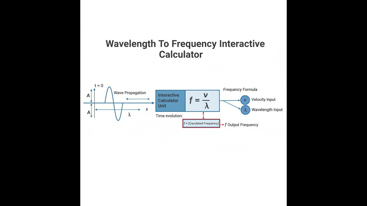
Wavelength To Frequency Interactive Calculator

Primary Wave Relationship

c = λf

f = c / λ

λ = c / f

Related Wave Parameters

Period: T = 1 / f

Angular Frequency: ω = 2πf

Wavenumber: k = 2π / λ

Photon Energy: E = hf = hc / λ

Variable Definitions:

• c = wave velocity (m/s) — speed of light in vacuum = 2.998 × 10⁸ m/s
• λ = wavelength (m) — spatial period of the wave
• f = frequency (Hz) — number of oscillations per second
• T = period (s) — time for one complete oscillation
• ω = angular frequency (rad/s) — rate of phase change
• k = wavenumber (rad/m) — spatial frequency
• E = photon energy (J) — quantum energy of electromagnetic radiation
• h = Planck's constant = 6.626 × 10^-34 J·s

The fundamental equation c = λf always holds, but the wave velocity c changes when electromagnetic radiation enters a material medium. In vacuum, c equals the universal constant 2.998 × 10⁸ m/s. In materials, the effective velocity becomes c/n where n is the refractive index. For visible light in glass (n ≈ 1.5), waves propagate at 2.0 × 10⁸ m/s, reducing wavelength by the factor n while frequency remains constant. This occurs because frequency is determined by the source oscillation rate and cannot change at the boundary, but the wave must slow down as it interacts with atomic electrons in the medium. The wavelength adjusts proportionally to maintain the wave equation. Dispersion arises because n varies with frequency, making different colors travel at different speeds and creating the chromatic effects seen in prisms and limiting optical fiber bandwidth to approximately 40 THz in the C-band window.

Penetration depth in conductive and dielectric materials follows fundamentally different wavelength dependencies. In metals, the skin depth δ = √(2/ωμσ) shows that longer wavelengths (lower frequencies) penetrate deeper: at 1 MHz in copper, δ = 66 μm, while at 1 GHz, δ = 2.1 μm—a 31× reduction. This makes low-frequency signals preferable for through-metal communication like submarine VLF transmissions at 20 kHz (λ = 15 km) that penetrate seawater to 30-meter depths, whereas microwave signals (λ = 3 cm) attenuate within centimeters. In dielectric materials like concrete or biological tissue, attenuation generally increases with frequency roughly as f^0.5 to f^2 depending on the loss mechanism. Water absorption peaks sharply at 22 GHz (λ = 13.6 mm) due to molecular rotational resonance, creating a local maximum where 5G millimeter-wave signals at 28 GHz (λ = 10.7 mm) experience 10-15 dB/km atmospheric attenuation from humidity, compared to 0.5 dB/km at 2.4 GHz (λ = 12.5 cm) where wavelength is far from resonance.

Measurement precision is ultimately limited by quantum uncertainty and practical instrumentation constraints. The Heisenberg uncertainty principle ΔE·Δt ≥ ħ/2 imposes a fundamental limit: a photon measured over time Δt has minimum energy uncertainty ΔE = ħ/(2Δt), creating frequency uncertainty Δf = 1/(4πΔt). For a 1 nanosecond measurement window, minimum frequency uncertainty is approximately 80 MHz. Spectral linewidth broadening from finite measurement time creates the Fourier-transform-limited resolution. Practically, wavemeters achieve 10 MHz precision (Δλ ≈ 0.00003 nm at 1550 nm) using Michelson interferometers with 15-meter path differences. Frequency counters reach 10⁻¹² fractional frequency stability over one-second averaging using atomic clock references, enabling wavelength determination to 0.0000015 nm at optical frequencies. Temperature variations cause refractive index changes of dn/dT ≈ 10⁻⁵ /°C in air, requiring ±0.1°C environmental control for sub-MHz wavelength stability measurements. The most precise measurements use frequency combs locked to cesium standards, achieving 10⁻¹⁵ fractional accuracy by directly counting optical cycles.

Relative motion between source and observer shifts both wavelength and frequency while maintaining c = λf in each reference frame, but the observed values differ from the emitted values. For non-relativistic velocities (v << c), the Doppler shift follows f_observed = f_source × (1 ± v/c) where positive sign indicates approach and negative indicates recession. A police radar at 24.15 GHz (λ = 12.41 mm) detecting a vehicle approaching at 30 m/s (108 km/h) measures a reflected frequency shift of Δf = 2 × 24.15 GHz × (30/2.998×10⁸) = 4.826 kHz, where the factor of 2 accounts for the round-trip Doppler effect. At relativistic velocities, the full formula f_obs = f_source × √[(1-β)/(1+β)] applies where β = v/c. For astronomical observations, galaxy recession velocities approaching 0.1c shift the hydrogen 21-cm line (1420.4 MHz) to 1551 MHz, a 130 MHz shift requiring precise wavelength-frequency conversion to determine redshift z = Δλ/λ = 0.0920, corresponding to a lookback time of 1.2 billion years using Hubble's law.

Antenna resonance conditions arise from electromagnetic boundary conditions that depend on physical dimensions relative to wavelength, not absolute time scales. A half-wave dipole resonates when its length L = λ/2 because current distribution must satisfy zero current at the ends and maximum current at the center—boundary conditions determined by spatial wave periodicity. At resonance, the antenna input impedance becomes purely real (typically 73Ω for a thin dipole), enabling efficient power transfer from transmission lines. Using frequency directly would give L = c/(2f), but this assumes propagation in vacuum. When antennas include dielectric loading or operate near ground planes, effective wavelength shortens by the velocity factor (0.95-0.97 for metal elements, 0.66 for coaxial cables), making wavelength the correct design parameter. For a cellular antenna at 1.9 GHz, free-space λ = 157.9 mm gives theoretical L = 78.95 mm, but practical ground-plane monopoles use 0.95 × (λ/4) = 37.5 mm accounting for velocity factor. Broadband antennas like log-periodic arrays maintain constant electrical dimensions by scaling physical size with wavelength across frequency ranges exceeding 10:1, demonstrating that λ determines electromagnetic scaling while f sets the operational band.

In dispersive media, different frequency components of a pulse travel at different group velocities, causing temporal spreading that cannot be characterized by a single wavelength-frequency conversion. The dispersion parameter β₂ = d²k/dω² determines pulse broadening rate, where k = 2π/λ is the wavenumber. For Gaussian pulses with initial duration τ₀ and spectral width Δω, propagation distance L produces temporal broadening to τ = τ₀√[1 + (β₂LΔω²/τ₀²)²]. A 100-femtosecond pulse at 800 nm (Δλ ≈ 13 nm, Δω ≈ 9.7 × 10¹³ rad/s) propagating through 10 mm of fused silica with β₂ = +36 fs²/mm experiences broadening to approximately 1.2 picoseconds—a 12× expansion. This occurs because the 13 nm spectral bandwidth contains wavelengths from 793.5 nm to 806.5 nm (corresponding to frequencies from 377.8 THz to 372.0 THz), and these components accumulate differential group delays of Δt = β₂ × L × Δω ≈ 1.1 ps. Wavelength-dependent velocity in the material creates frequency chirp where instantaneous frequency sweeps across the pulse duration, requiring either dispersion compensation using chirped mirrors or mathematical wavelength-to-frequency mapping accounting for β₂ to recover original pulse characteristics. Fiber-optic communication systems operating at 10 Gb/s with 100-picosecond bit periods must limit dispersion-induced spreading below 10 ps, constraining transmission distance-bandwidth products based on precise wavelength-to-group-velocity conversion using the material dispersion curve D(λ).

Free Engineering Calculators

Explore our complete library of free engineering and physics calculators.

🔗 Explore More Free Engineering Calculators

• Optical Encoder Index Pulse Timing Calculator
• Lens Focal Length & Working Distance Solver
• Angular Resolution Calculator
• Wavelength To Energy Calculator
• Frequency Bandwidth Calculator

Browse All Engineering Calculators →

About the Author

Robbie Dickson — Chief Engineer & Founder, FIRGELLI Automations

Robbie Dickson brings over two decades of engineering expertise to FIRGELLI Automations. With a distinguished career at Rolls-Royce, BMW, and Ford, he has deep expertise in mechanical systems, actuator technology, and precision engineering.

Wikipedia · Full Bio