Frequency To Wavelength Interactive Calculator

The Frequency to Wavelength Interactive Calculator converts between the frequency and wavelength of electromagnetic or mechanical waves traveling through various media. This relationship is fundamental to telecommunications engineering, radio frequency design, fiber optics, acoustic engineering, and spectroscopy. Understanding wavelength-frequency relationships enables engineers to design antennas, optical systems, acoustic transducers, and RF circuits optimized for specific propagation characteristics.

📐 Browse all free engineering calculators

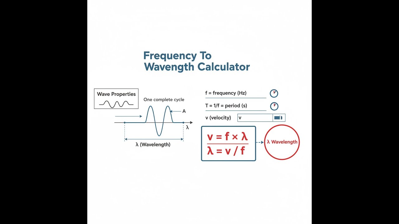
Wave Propagation Diagram

Interactive Frequency-Wavelength Calculator

Fundamental Equations

Theory & Practical Applications

The Universal Wave Relationship

The relationship v = f × λ represents one of the most fundamental principles in physics, governing all wave phenomena from seismic waves with wavelengths measured in kilometers to gamma rays with wavelengths smaller than atomic nuclei. This equation encodes the deep connection between temporal oscillation (frequency) and spatial periodicity (wavelength), mediated by the propagation velocity characteristic of the medium.

For electromagnetic waves in vacuum, the velocity is exactly c = 299,792,458 m/s, a fundamental constant that defines the meter in the SI system. This invariance underpins special relativity and represents the maximum speed at which information can propagate through space. In material media, electromagnetic waves propagate more slowly due to interactions with atomic electrons, leading to the phenomenon of refraction and the definition of the refractive index n = c/v.

What's less obvious but critically important for engineering applications is that frequency remains constant across media boundaries while wavelength adjusts proportionally to the velocity change. When light passes from air (n ≈ 1.0003) into glass (n ≈ 1.5), its wavelength decreases by a factor of 1.5 while its frequency remains exactly the same. This invariance of frequency is what allows fiber optic communications to work — the information encoded in frequency modulation is preserved despite multiple reflections and material transitions within the fiber core.

Electromagnetic Spectrum Engineering

The electromagnetic spectrum spans more than 20 orders of magnitude in frequency, from extremely low frequency (ELF) radio waves at 3 Hz (wavelength ≈ 100,000 km) to ultra-high-energy gamma rays beyond 10²⁴ Hz (wavelength smaller than 10^-16 m). Each region exhibits unique propagation characteristics that dictate engineering applications.

Radio frequencies (RF) below 3 GHz can diffract around obstacles and penetrate buildings, making them ideal for mobile communications. The specific allocation of cellular bands (e.g., 850 MHz, 1.9 GHz, 2.4 GHz, 5 GHz) represents careful engineering tradeoffs between antenna size (λ/4 monopoles are practical), propagation range (lower frequencies propagate farther), and available bandwidth (higher frequencies support more data).

Microwave frequencies (300 MHz to 300 GHz) enable radar, satellite communications, and microwave ovens. The 2.45 GHz frequency chosen for microwave ovens corresponds to a wavelength of 12.2 cm, selected because it efficiently excites rotational modes of water molecules while allowing reasonably compact cavity dimensions. Modern 5G networks increasingly use millimeter wave bands (24-47 GHz) where wavelengths of 6-12 mm enable massive antenna arrays (hundreds of elements) to be packed into small physical volumes for beamforming.

Infrared wavelengths (700 nm to 1 mm) are critical for thermal imaging and fiber optic communications. The telecommunications windows at 1310 nm and 1550 nm represent local minima in the attenuation spectrum of silica fiber — wavelengths where propagation losses drop to just 0.2-0.3 dB/km, enabling 100+ km transmission distances without amplification.

Visible light (380-700 nm) represents the narrow band to which our eyes evolved sensitivity, matching the peak intensity of solar radiation at Earth's surface. This is not coincidence but evolutionary optimization. Engineering applications include photolithography (using 193 nm deep-UV for sub-7nm semiconductor nodes), colorimetry (CIE standard observer functions), and visible light communications (VLC) achieving multi-Gbps data rates.

Acoustic Wave Applications

Sound waves in air at 20°C propagate at approximately 343 m/s, far slower than electromagnetic waves and resulting in much longer wavelengths at comparable frequencies. A 1 kHz sound wave has wavelength λ = 343/1000 = 0.343 m = 34.3 cm, which determines the behavior of acoustic systems.

Loudspeaker design is fundamentally constrained by wavelength. A driver radiates omnidirectionally when its diameter D is much smaller than the wavelength (D < λ/2), but becomes increasingly directional as frequency increases and λ becomes comparable to D. This is why most speaker systems employ small tweeters for high frequencies (short wavelengths requiring small radiating area) and large woofers for low frequencies (long wavelengths requiring large displacement area). A 12-inch woofer (30 cm diameter) becomes directional above approximately 570 Hz where λ = 60 cm.

Room acoustics are dominated by wavelength-dimension interactions. Bass frequencies below 80 Hz (λ > 4.3 m) create standing wave modes in typical rooms, resulting in severe spatial variation in low-frequency response. This is why subwoofer placement is so critical — you're physically positioning the source within the three-dimensional resonant cavity formed by the room boundaries. Modal analysis using the equation f_n,m,l = (c/2)√[(n/L_x)² + (m/L_y)² + (l/L_z)²] predicts exact frequencies where standing waves occur based on room dimensions.

Ultrasonic applications exploit frequencies above human hearing (20 kHz+) where short wavelengths enable high spatial resolution. Medical ultrasound at 3-10 MHz (λ = 0.5-0.15 mm in tissue) achieves millimeter-scale imaging. Ultrasonic cleaning at 40 kHz (λ = 8.6 mm in water) creates cavitation bubbles for surface cleaning. Ultrasonic welding of plastics uses 20-40 kHz to generate localized heating at molecular interfaces.

Refractive Index and Dispersion

The refractive index n is not a single constant but a frequency-dependent function n(f) that varies due to atomic and molecular resonances in the material. This phenomenon, called dispersion, causes different wavelengths to propagate at different velocities, leading to chromatic aberration in lenses and pulse broadening in optical fibers.

Normal dispersion occurs far from material resonances where dn/dλ > 0 (refractive index increases with decreasing wavelength). This is why prisms separate white light with blue light (shorter wavelength) bending more than red light (longer wavelength). Typical visible-spectrum glasses have refractive indices ranging from n ≈ 1.51 at 700 nm (red) to n ≈ 1.53 at 400 nm (violet), a variation that may seem small but produces significant chromatic aberration over the focal length of telephoto lenses.

Optical fiber dispersion limits data transmission rates because different wavelengths within a pulse travel at different group velocities, causing pulse spreading that eventually merges adjacent bits. Standard single-mode fiber exhibits zero-dispersion at 1310 nm, which is why this wavelength was historically preferred for long-distance telecommunications. Modern dispersion-shifted fibers and wavelength-division multiplexing (WDM) systems carefully engineer the dispersion profile across the C-band (1530-1565 nm) to minimize pulse spreading while avoiding four-wave mixing nonlinearities.

Antenna Design and Wavelength Scaling

Antenna dimensions scale directly with wavelength, making frequency selection a critical systems engineering decision. A half-wave dipole antenna has length L = λ/2, so a 100 MHz antenna requires L = 1.5 m while a 2.4 GHz antenna requires only L = 6.25 cm. This is why WiFi routers can have compact internal antennas while AM broadcast stations require massive tower arrays.

The practical implication extends beyond just size. Antenna gain scales as G ∝ (D/λ)² for an aperture antenna of diameter D, meaning that achieving high gain at low frequencies requires physically enormous structures. A 30 dBi (1000× power gain) antenna at 100 MHz requires a dish approximately 15 meters in diameter, while the same gain at 10 GHz requires only 15 cm — explaining why satellite dishes for Ku-band (12 GHz) can be compact consumer products.

Phased array antennas for 5G applications exploit the millimeter-wave bands (28 GHz, λ = 10.7 mm) where antenna element spacing of λ/2 = 5.4 mm allows 64 or 128 elements to fit in a smartphone-sized array. The beamwidth of such an array is approximately θ ≈ λ/(N·d) radians where N is the number of elements and d is the spacing, enabling electronically steerable beams with sub-degree precision for massive MIMO (multiple-input multiple-output) communications.

Worked Example: Multi-Band Antenna System Design

A telecommunications company is designing a multi-band cellular tower that must support three frequency bands simultaneously: LTE Band 12 (700 MHz), LTE Band 2 (1900 MHz), and 5G n77 (3.7 GHz). Calculate the required dipole antenna lengths for each band, the relative size difference between the lowest and highest frequency antennas, and determine the optimal wavelength spacing for a 16-element linear phased array operating at 3.7 GHz.

Given Information:

• Band 12 center frequency: f₁ = 700 MHz
• Band 2 center frequency: f₂ = 1900 MHz
• 5G n77 center frequency: f₃ = 3.7 GHz
• Wave propagation velocity (EM waves in air): c = 299,792,458 m/s ≈ 3 × 10⁸ m/s
• Phased array specifications: 16 elements, linear configuration

Step 1: Calculate wavelengths for each band

Using λ = c / f:

Band 12 (700 MHz):
λ₁ = (3 × 10⁸ m/s) / (700 × 10⁶ Hz) = 0.4286 m = 42.86 cm

Band 2 (1900 MHz):
λ₂ = (3 × 10⁸ m/s) / (1900 × 10⁶ Hz) = 0.1579 m = 15.79 cm

5G n77 (3.7 GHz):
λ₃ = (3 × 10⁸ m/s) / (3.7 × 10⁹ Hz) = 0.08108 m = 8.108 cm

Step 2: Calculate half-wave dipole antenna lengths

A practical half-wave dipole has length L = λ/(2 × velocity_factor). For wire antennas in air, the velocity factor is approximately 0.95 due to end effects, giving L = 0.475λ:

Band 12 dipole length:
L₁ = 0.475 × 42.86 cm = 20.36 cm ≈ 20.4 cm

Band 2 dipole length:
L₂ = 0.475 × 15.79 cm = 7.50 cm

5G n77 dipole length:
L₃ = 0.475 × 8.108 cm = 3.85 cm

Step 3: Calculate size ratios

Ratio of longest to shortest antenna:
L₁/L₃ = 20.36 / 3.85 = 5.29

The 700 MHz antenna is 5.29 times longer than the 3.7 GHz antenna, corresponding exactly to the frequency ratio: 3700/700 = 5.29. This demonstrates the inverse proportionality between frequency and antenna dimensions.

Step 4: Phased array element spacing for 3.7 GHz

For a phased array to avoid grating lobes (unwanted beams), element spacing must satisfy d ≤ λ/(1 + |sin θ_max|) where θ_max is the maximum scan angle. For ±60° scanning capability:

d_max = λ₃ / (1 + sin 60°) = 8.108 cm / (1 + 0.866) = 8.108 / 1.866 = 4.345 cm

A standard design uses d = λ/2 = 4.054 cm, which safely avoids grating lobes while maximizing aperture size.

Step 5: Calculate total array aperture and beamwidth

Total array length for 16 elements:
L_array = 15 × d = 15 × 4.054 cm = 60.81 cm (the first element doesn't add spacing)

The theoretical 3 dB beamwidth for a uniformly illuminated linear array is:
θ_3dB ≈ 0.886 × λ / L_array = 0.886 × 8.108 cm / 60.81 cm = 0.1182 radians = 6.77°

Engineering Implications:

This example reveals several critical design constraints. The 5.29× size difference between 700 MHz and 3.7 GHz antennas means that tower space is dominated by low-frequency elements, often requiring separate mounting positions. The 3.7 GHz phased array, despite having 16 elements, occupies only 60.81 cm, enabling compact massive MIMO panels that can be building-mounted rather than requiring dedicated towers.

The 6.77° beamwidth at 3.7 GHz provides high spatial selectivity, allowing the same physical tower to serve multiple users in different angular directions through beamforming — effectively multiplying capacity without adding spectrum. This is impossible at 700 MHz where the equivalent beamwidth would be 35.8°, requiring 5.29× more elements (85 elements) to achieve the same angular resolution, which becomes mechanically and economically impractical.

This fundamental wavelength-antenna size relationship drives the entire architecture of modern cellular networks, where low-frequency bands provide coverage and high-frequency bands provide capacity through spatial multiplexing.

Practical Measurement Considerations

Frequency and wavelength measurements require different techniques across the electromagnetic spectrum. At radio frequencies below 1 GHz, frequency counters directly measure the number of zero-crossings per second with precision exceeding 1 Hz in 1 MHz (parts-per-million accuracy). This is how GPS receivers achieve centimeter-level positioning by comparing carrier frequencies to atomic clock references.

At optical frequencies (hundreds of THz), direct frequency counting is impossible with electronic circuits. Instead, wavelength meters use interferometry to measure λ by comparing path length differences, then calculate frequency from f = c/λ. Modern wavemeters achieve 1 part in 10⁷ accuracy, sufficient for wavelength-division multiplexing where channels are spaced by 100 GHz (≈0.8 nm at 1550 nm).

The transition between electronic and photonic measurement techniques occurs around 100 GHz, where both approaches reach practical limits. This "terahertz gap" represents a challenging region for instrumentation, though recent advances in photoconductive antenna technology and quantum cascade lasers are closing this window for applications including security scanning and molecular spectroscopy.

Frequently Asked Questions