Production Rate Units Hour Interactive Calculator

Production rate calculation is fundamental to manufacturing efficiency, capacity planning, and cost analysis. This interactive calculator helps manufacturing engineers, production managers, and industrial planners determine production rates, cycle times, required production hours, and the number of machines needed to meet output targets across various production scenarios.

📐 Browse all free engineering calculators

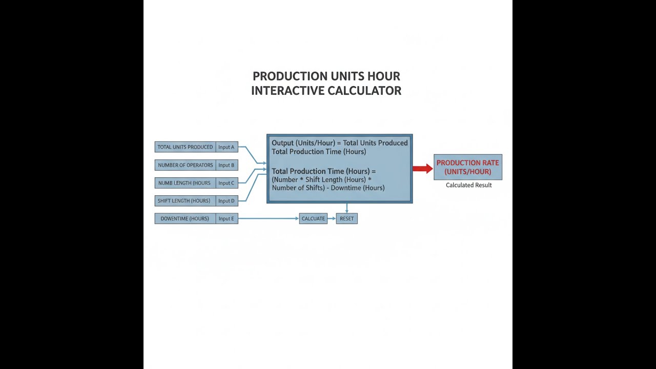
Production Rate System Diagram

Production Rate Calculator

Production Rate Equations

Theory & Engineering Applications

Production rate calculation forms the foundation of manufacturing engineering, industrial capacity planning, and operational efficiency analysis. Understanding production rates enables manufacturers to accurately forecast output, plan resource allocation, identify bottlenecks, and measure equipment effectiveness. These calculations are critical across industries from automotive assembly to pharmaceutical manufacturing, semiconductor fabrication to food processing.

Fundamental Production Rate Theory

Production rate represents the throughput of a manufacturing system, typically expressed as units produced per unit of time. While the basic calculation divides total output by total time, real-world production environments introduce complexity through variability in cycle times, equipment downtime, changeover periods, and quality defects. The distinction between theoretical maximum rate and actual achieved rate reveals critical information about system constraints and improvement opportunities.

Cycle time, the inverse of production rate when normalized to consistent time units, represents the time interval between consecutive unit completions. In high-volume manufacturing, cycle time variations of even a few seconds compound into significant capacity differences over a production shift. This relationship becomes particularly important in synchronized production systems where one slow operation creates a bottleneck affecting the entire line.

Takt Time vs. Cycle Time: A Critical Distinction

One frequently misunderstood concept in production rate analysis is the relationship between takt time and cycle time. Takt time represents the rate at which products must be produced to meet customer demand, calculated by dividing available production time by customer demand. For a factory operating 28,800 seconds per day (8 hours) with customer demand of 576 units, the takt time is 50 seconds per unit. This differs fundamentally from cycle time, which measures actual production speed.

For efficient production, cycle time must equal or be less than takt time. When cycle time exceeds takt time, production cannot meet demand without overtime or additional capacity. This relationship drives lean manufacturing principles where processes are balanced to match takt time, eliminating waste from both overproduction and capacity shortages.

Overall Equipment Effectiveness (OEE)

OEE provides a comprehensive measure of manufacturing productivity by incorporating three dimensions: availability (uptime percentage), performance (speed compared to ideal), and quality (good units as percentage of total). A machine with 90% availability, 95% performance, and 98% quality achieves an OEE of 83.8% (0.90 × 0.95 × 0.98). World-class manufacturing typically targets OEE above 85%, while many facilities operate between 60-70%.

The multiplicative nature of OEE reveals how seemingly small losses in each dimension compound dramatically. A 5% loss in availability, 5% in performance, and 2% in quality results in 11.5% total capacity loss, not 12%. This non-linear relationship emphasizes the importance of addressing all three factors simultaneously rather than focusing on a single dimension.

Multi-Machine Production Systems

Calculating required machine count involves ceiling functions rather than simple division because fractional machines cannot exist. If production requires 3.2 machines based on rate calculations, four machines must be deployed. This creates inherent overcapacity that can serve as buffer capacity, support preventive maintenance schedules, or accommodate demand growth. Machine utilization percentage (required machines / actual machines × 100) quantifies this excess capacity.

In parallel machine configurations, total system rate equals the sum of individual machine rates only when machines operate identically and independently. Real systems introduce complications through shared resources, material handling constraints, and quality control bottlenecks. These factors often limit actual combined throughput to 85-95% of the theoretical sum of individual rates.

Production Rate Variability and Buffer Sizing

All production processes exhibit variability in cycle times, creating challenges for capacity planning and scheduling. The coefficient of variation (standard deviation divided by mean cycle time) quantifies this variability. High variability necessitates larger buffer inventories between production stages to prevent starvation of downstream operations. Queueing theory demonstrates that utilization above 80-85% in variable systems leads to exponentially increasing wait times and work-in-process inventory.

This relationship explains why theoretical capacity calculations often overestimate actual achievable throughput. A line designed for 100 units per hour may realistically achieve only 80-85 units per hour in sustained operation when accounting for variability, minor stoppages, and material handling delays. Experienced production planners typically apply safety factors of 15-25% when converting theoretical rates to production commitments.

Worked Example: Complete Production Planning Analysis

Consider an electronics manufacturer planning production of a new circuit board assembly. Marketing projects demand of 12,000 units per month. The factory operates two 8-hour shifts, five days per week (approximately 22 working days per month). Initial pilot production achieved 47 units over a 4-hour test run with 3 defective units.

Step 1: Calculate demonstrated production rate
Production rate = 47 units / 4 hours = 11.75 units/hour
Quality rate = (47 - 3) / 47 = 93.6%
Good unit production rate = 11.75 × 0.936 = 11.00 good units/hour

Step 2: Calculate monthly capacity requirement
Available production hours per month = 22 days × 16 hours/day = 352 hours
Required production rate = 12,000 units / 352 hours = 34.09 units/hour
With 93.6% quality rate, required gross rate = 34.09 / 0.936 = 36.43 units/hour

Step 3: Determine machine requirements
Machines required = 36.43 units/hour ÷ 11.75 units/hour per machine = 3.10 machines
Actual machines needed = 4 machines (rounded up)
Machine utilization = 3.10 / 4 = 77.5%

Step 4: Calculate actual capacity and OEE
Actual production capacity = 4 machines × 11.00 good units/hour × 352 hours = 15,488 good units/month
Capacity surplus = 15,488 - 12,000 = 3,488 units (29.1% buffer)
If we assume 85% availability factor for planned maintenance: Effective capacity = 15,488 × 0.85 = 13,165 units/month
OEE estimation = 85% availability × 77.5% performance × 93.6% quality = 61.6%

Step 5: Identify improvement opportunities
To achieve world-class OEE of 85%, the manufacturer could:
- Improve quality to 98% (reducing defect rate from 6.4% to 2%): gains 4.4% capacity
- Increase availability to 90% through better maintenance: gains 5% capacity
- Reduce cycle time to 4.9 minutes/unit (from 5.1): gains 4% performance
Combined improvements could raise capacity to 17,250 units/month with same equipment

This analysis reveals that purchasing four machines with 77.5% utilization provides adequate buffer capacity for the 12,000 unit demand while allowing for maintenance, quality issues, and demand fluctuations. The relatively low OEE of 61.6% indicates substantial improvement potential before additional capital investment becomes necessary.

Industry-Specific Applications

In automotive manufacturing, production rate calculations determine assembly line speed, which typically operates at fixed takt times between 45-90 seconds per vehicle depending on plant size and model complexity. Every station must complete its work within the takt time, requiring precise balancing of work content across stations. A single station exceeding takt time creates a bottleneck limiting entire plant output.

Pharmaceutical manufacturing faces unique constraints where batch processing rather than continuous flow dominates. Production rate calculations must account for batch setup time, processing time, cleaning validation, and quality hold times. A tablet press might achieve 300,000 tablets per hour during compression but only 180,000 tablets per hour when amortizing changeover and cleaning across batch size.

Semiconductor fabrication represents the most capital-intensive production environment, where equipment costs millions of dollars per tool and cycle times span hours to days. Fab capacity planning uses wafer starts per week as the primary metric, with complex calculations accounting for rework rates, equipment dedication to specific products, and preventive maintenance schedules reducing availability to 75-85%.

For more manufacturing and quality calculators, visit our engineering calculator library.

Practical Applications

Frequently Asked Questions