Hydraulic Conductivity Interactive Calculator

Hydraulic conductivity quantifies how easily water flows through porous media like soil, rock, or geotextiles under a hydraulic gradient. This calculator solves for hydraulic conductivity (K), discharge velocity (q), hydraulic gradient (i), or cross-sectional area (A) using Darcy's Law, the fundamental equation governing groundwater flow, contaminant transport modeling, and subsurface drainage design across geotechnical engineering, hydrogeology, and environmental remediation projects.

📐 Browse all free engineering calculators

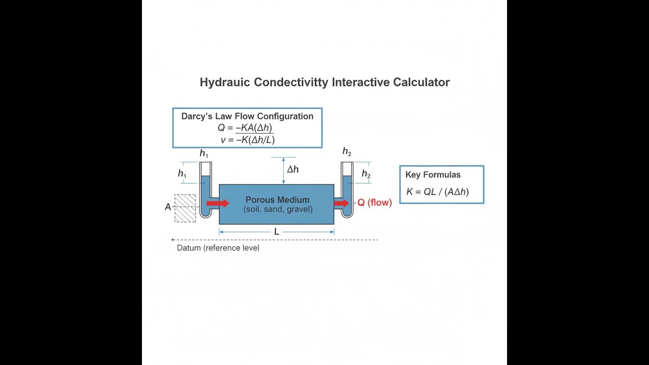
System Diagram: Hydraulic Flow Through Porous Media

Hydraulic Conductivity Calculator

Governing Equations

Theory & Practical Applications

Fundamental Physics of Darcy's Law

Darcy's Law, formulated by French engineer Henry Darcy in 1856 through experimental studies of water flow through sand filters, describes the empirical relationship between fluid discharge velocity and hydraulic gradient in porous media. The law applies to laminar flow conditions where Reynolds number (Re) is less than approximately 1-10, depending on pore geometry. Beyond this critical Reynolds number, turbulent effects dominate and Darcy's Law breaks down — a regime often encountered in fractured rock aquifers or coarse gravel deposits where the Forchheimer equation becomes necessary.

The hydraulic conductivity K is not merely a property of the porous medium alone; it is a composite parameter incorporating both the intrinsic permeability of the material (a purely geometric property related to pore size and connectivity) and the fluid properties (density and dynamic viscosity). The relationship is expressed as K = (k·ρ·g)/μ, where k is intrinsic permeability [m²], ρ is fluid density [kg/m³], g is gravitational acceleration [m/s²], and μ is dynamic viscosity [Pa·s]. This distinction becomes critical when dealing with non-water fluids (petroleum products, NAPL contaminants) or temperature-dependent flow scenarios where viscosity changes significantly.

Scale Effects and Heterogeneity in Real Systems

Laboratory-measured hydraulic conductivity values frequently differ by one to three orders of magnitude from field-scale effective conductivity. This discrepancy arises from spatial heterogeneity — natural geologic formations exhibit layering, lenses of contrasting materials, and anisotropy (directional dependence of K). Horizontal hydraulic conductivity (K_h) typically exceeds vertical conductivity (K_v) by factors of 3 to 100 in sedimentary deposits due to preferential horizontal bedding planes. Engineers must account for this through careful site characterization using multiple-scale testing: slug tests for local values, pumping tests for aquifer-scale averages, and tracer tests for transport-relevant effective conductivity.

A common error in groundwater modeling is applying isotropic conductivity assumptions to stratified aquifers. Consider a three-layer system where sand (K=1×10⁻⁴ m/s), clay (K=1×10⁻⁸ m/s), and gravel (K=1×10⁻² m/s) layers each occupy one-third of the aquifer thickness. For horizontal flow, the effective K_h is the arithmetic mean weighted by thickness. For vertical flow, the effective K_v is the harmonic mean — dominated by the least permeable layer. The result: K_h/K_v can exceed 10,000, fundamentally altering contaminant migration pathways.

Engineering Applications Across Disciplines

Groundwater Resource Management: Municipal water supply wells abstract groundwater at rates governed by the aquifer's transmissivity (T = K·b, where b is aquifer thickness). The Theis solution and Jacob's approximation for transient well hydraulics both build upon Darcy's Law to predict drawdown cones and sustainable yield. Overextraction leads to land subsidence — Mexico City has subsided over 10 meters since 1900 due to excessive pumping from confined aquifers with hydraulic conductivities in the range 10⁻⁶ to 10⁻⁵ m/s.

Environmental Remediation: CERCLA Superfund sites rely on pump-and-treat systems designed using Darcy-based capture zone analysis. Dense non-aqueous phase liquids (DNAPLs) like chlorinated solvents sink through aquifers until encountering low-K barriers. Predicting DNAPL migration requires modified Darcy formulations accounting for multiphase flow and interfacial tensions — the relative permeability becomes a function of saturation state. Permeable reactive barriers (PRBs) containing zero-valent iron depend on sufficient hydraulic conductivity (typically K > 10⁻⁴ m/s) to ensure adequate contact time between contaminated groundwater and reactive media.

Dam and Levee Seepage Analysis: Earthen embankment dams experience seepage-induced pore pressures that reduce effective stress and potentially trigger failure. Flow net construction using Darcy's Law determines the phreatic surface location and exit gradients. Critical hydraulic gradients (i_crit ≈ 1.0 for uniform sands) mark the threshold for piping failure — a phenomenon responsible for approximately 40% of historical dam failures worldwide. Seepage cutoff walls (slurry walls with K < 10⁻⁹ m/s) or grouting programs reduce seepage rates by introducing low-conductivity barriers.

Agricultural Drainage Design: Subsurface tile drains spaced according to the Hooghoudt equation prevent waterlogging in irrigated fields. The equation incorporates hydraulic conductivity, drain depth, and spacing to maintain water table levels below the root zone. Poorly drained soils (K < 10⁻⁷ m/s) require closer drain spacing (3-10 meters), while well-drained sandy loams (K > 10⁻⁵ m/s) function adequately with 20-50 meter spacing. More information on related engineering calculations can be found in the broader engineering calculator library.

Worked Example: Dewatering System Design

Problem Statement: A 12-meter-deep excavation for an underground parking structure requires dewatering in a confined aquifer with the following characteristics: hydraulic conductivity K = 4.7×10⁻⁴ m/s (medium sand), aquifer thickness b = 18 meters, initial piezometric surface at ground level. Determine: (a) the required pumping rate Q from a single well to lower the water table 3.2 meters below excavation base at a radial distance of 24 meters, (b) the hydraulic gradient at the well screen, (c) the seepage velocity assuming porosity n = 0.35, and (d) the drawdown at the excavation perimeter.

Solution:

Part (a): Pumping Rate Using Thiem Equation (Steady-State)

For a confined aquifer with fully penetrating well, the Thiem equation relates pumping rate to drawdown:

Q = (2πKb(h₁ - h₂)) / ln(r₁/r₂)

Where h₁ and h₂ are hydraulic heads at radii r₁ and r₂ from the pumping well. We need 3.2 m drawdown at r₁ = 24 m (excavation radius), and assume radius of influence r₂ = 300 m (typical for medium sand) where drawdown is negligible.

h₁ = 18 - 3.2 = 14.8 m (head at excavation perimeter)
h₂ = 18 m (head at radius of influence)
Δh = 18 - 14.8 = 3.2 m

Q = (2π × 4.7×10⁻⁴ m/s × 18 m × 3.2 m) / ln(300/24)
Q = (1.696×10⁻¹ m³/s) / 2.526
Q = 6.71×10⁻² m³/s = 67.1 L/s = 1,062 gallons per minute

Part (b): Hydraulic Gradient at Well Screen (r_w = 0.3 m)

The discharge velocity at any radius r is given by Q = 2πrbq, where q = K·i. Rearranging for gradient:

i = Q / (2πrbK)

At the well screen radius r_w = 0.3 m:

i = (6.71×10⁻² m³/s) / (2π × 0.3 m × 18 m × 4.7×10⁻⁴ m/s)
i = (6.71×10⁻²) / (1.595×10⁻²)
i = 4.21 (dimensionless)

This high gradient near the well screen is typical and demonstrates why well screen design must prevent sand pumping and maintain structural integrity under significant hydraulic forces.

Part (c): Seepage Velocity at Excavation Perimeter

First, calculate discharge velocity at r = 24 m:

q = Q / (2πrb) = (6.71×10⁻² m³/s) / (2π × 24 m × 18 m)
q = (6.71×10⁻²) / (2.714×10³)
q = 2.47×10⁻⁵ m/s

Seepage velocity (actual pore water velocity):

v_s = q / n = (2.47×10⁻⁵ m/s) / 0.35
v_s = 7.06×10⁻⁵ m/s = 6.10 m/day

This seepage velocity governs contaminant transport timescales if dewatering mobilizes dissolved pollutants.

Part (d): Drawdown at Well Location

Using the Thiem equation again with r₁ = r_w = 0.3 m:

s_w = Q·ln(r₂/r_w) / (2πKb)
s_w = (6.71×10⁻² × ln(300/0.3)) / (2π × 4.7×10⁻⁴ × 18)
s_w = (6.71×10⁻² × 6.908) / (5.340×10⁻²)
s_w = 8.67 meters

This requires the well pump intake to be set below 18 - 8.67 = 9.33 m elevation to prevent cavitation. The analysis demonstrates how Darcy's Law, extended through classical well hydraulics, provides complete design parameters for dewatering systems — from pump sizing to monitoring well placement.

Non-Darcy Flow and Limitations

Three primary conditions violate Darcy's Law assumptions: (1) turbulent flow at high velocities where inertial forces become significant (Forchheimer equation required), (2) non-Newtonian fluids such as drilling muds or polymer-amended groundwater, and (3) two-phase flow during oil recovery or air sparging remediation where relative permeability functions replace the single-phase K value. In fractured rock, discrete fracture network (DFN) modeling supersedes continuum Darcy formulations because flow is concentrated in high-conductivity fractures (K_fracture > 10⁻² m/s) separated by low-conductivity matrix (K_matrix < 10⁻¹⁰ m/s). The equivalent porous medium approach fails catastrophically in such settings — a lesson learned from numerous failed remediation attempts at fractured bedrock sites.

Frequently Asked Questions