Friction Loss Interactive Calculator

If you ignore friction losses in a mechanical system, you risk undersizing your motors, generating heat in unexpected places, and missing efficiency targets. The Friction Loss Interactive Calculator here lets you work out friction force, coefficient of friction, normal force, or power loss using realistic figures—mass, velocity, surface coefficient, and incline angle. These values aren’t just paperwork—they affect power draw and heat generation in machines like conveyors, brakes, and actuator systems. The page gives you core formulas, a step-by-step conveyor example, practical friction discussion, and plain answers to real-world questions.

What is friction loss?

Friction loss is the energy burned up when two surfaces slide over one another. It turns into heat, slows things down, and forces your motor to work harder than if there were no friction at all.

Simple Explanation

If you’ve ever pushed a heavy box across a floor, you’ll know rough floors need more effort. That extra push is friction loss. Push two things together harder, or use rougher surfaces, and you’ll spend more energy overcoming friction rather than getting useful work out the other side—it mostly becomes heat.

📐 Browse all 1000+ Interactive Calculators

Friction Force Diagram

How to Use This Calculator

1. Pick which result you need (friction force, coefficient, normal force, power loss, incline friction, or stopping distance) from the dropdown menu.
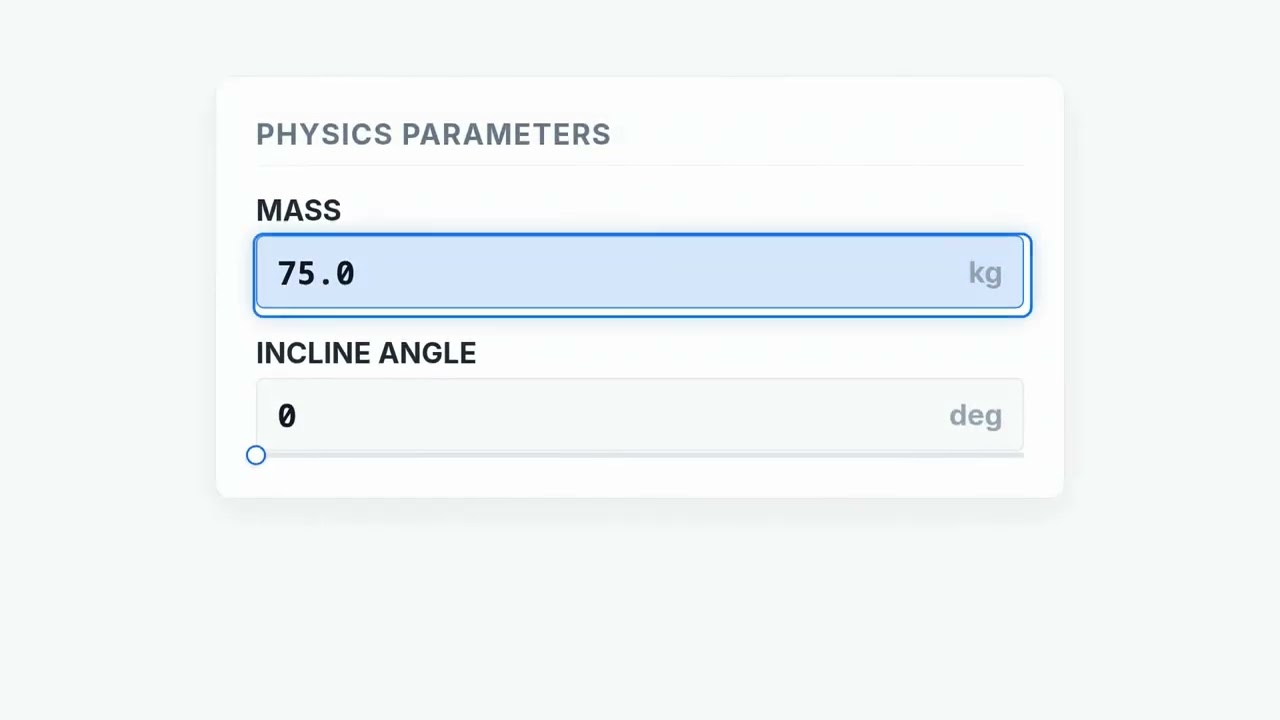
2. Input your values as needed—coefficient, normal force, mass, velocity, or incline angle, depending on the calculation.
3. If you want to see a sample, hit "Try Example" to load preset data and see what happens.
4. Press Calculate to get your number.

Friction Loss Interactive Calculator

Friction Equations

You’ll find the basic friction force with this equation:

To estimate power lost as friction, use:

Friction on inclines changes based on the angle. The equations:

For stopping distance problems, friction sets the minimum distance:

Simple Example

Suppose you have a 50 kg steel block on a horizontal surface with a coefficient of friction μ = 0.35.

• Normal force: F_N = 50 × 9.81 = 490.5 N
• Friction force: F_f = 0.35 × 490.5 = 171.7 N
• Power loss at 2 m/s: P = 171.7 × 2 = 343.4 W

Theory & Practical Applications

The Physics of Friction: Microscopic Origins and Macroscopic Models

On a microscopic level, friction comes from countless tiny surface peaks—asperities—touching, locking together, and deforming as the parts move. Even polished surfaces aren’t smooth at the scale where friction happens. Friction force is usually estimated with the classic Amontons-Coulomb law: F_f = μF_N. This keeps calculations manageable, but it leaves out a lot: it ignores contact area (because more area gives lower pressure, so the real atomic contact area remains about the same as force goes up); it skips chemical and temperature effects; it works “good enough” for most basic mechanical design. But don’t expect it to capture everything if you’re pushing the limits.

The coefficient of friction (μ) depends not just on the materials, but also how rough or worn the surfaces are, their temperature, if they’re contaminated, and sometimes the speed involved. Static friction coefficients are always higher than kinetic by around 10–50%, because things not yet moving can bond better at the contact points. That difference makes stick-slip effects—a real problem for slow and precise actuator positioning—especially at startup. At very low speeds, friction doesn’t stay constant: the Stribeck effect means it can shoot up, so low-speed actuator motion often needs special attention and sometimes different modeling.

Material Pairings and Surface Engineering

Real-world coefficients vary a lot. For example, PTFE (Teflon) on steel can be as low as μ ≈ 0.04, while dry steel-on-steel can be 0.6–0.8. Add lubrication and some bearings run at μ ≈ 0.02 for a basic bushing down to about 0.001 for a well-engineered ball bearing. On the other end, rubber on dry concrete might top μ = 1.2. Ra surface finish matters: two identical metals with one mirror-finished and the other only machined will have noticeably different friction, even at the same load and speed.

Designers use this to their advantage. In brakes, you want high friction—so you see sintered metal pads on iron rotors around μ = 0.35–0.45, and then deal with all the heat that results. In conveyors, you want low friction—use good bearings (μ ≈ 0.001–0.005) and you might only need a fraction of the motor power versus sliding friction (μ ≈ 0.6). For a 500 kg load on a long belt, switching to good bearings could cut loss from over 3 kW down to under 100 W, with real energy savings and easier thermal management.

Thermal Management and Temperature Effects

Friction invariably makes heat wherever significant force and speed come together: high-speed machines, brakes, actuators under heavy load. Power lost at the friction interface is simple to calculate—just F_f × v—but controlling temperature isn’t always easy. For instance, a linear rail with 800 N normal force and μ = 0.12, running 0.5 m/s, wastes nearly 50 W as heat. Without enough cooling or heat conduction to structure, component temperature can rise quickly.

Friction coefficients change with temperature and so do lubricants. Many plastics used in bushings will give you 15–30% higher μ at 80°C than at 20°C. Lubricating oils thin out with heat, making fluid films weaker and letting surfaces touch again, only adding to the problem. If your heat isn’t removed, you can get a run-away effect—parts get hotter, friction grows, then everything spirals up. Industrial actuators dealing with constant high loads and speed often need real cooling, not just passive metal housings.

Worked Example: Conveyor Belt Drive Motor Sizing

Say you need a conveyor to move 750 kg of steel parts 15 m across the shop floor, speed set at 0.8 m/s. Use steel rollers with effective μ = 0.018. Here’s the practical approach:

Step 1: Calculate Normal Force
The load's weight is the normal force:
F_N = m × g = 750 × 9.81 = 7357.5 N

Step 2: Calculate Total Friction Force
F_f = μ × F_N = 0.018 × 7357.5 = 132.4 N

Step 3: Calculate Mechanical Power Required
P_mechanical = F_f × v = 132.4 × 0.8 = 105.9 W

Step 4: Account for Motor and Drive Efficiency
Assume your motor is 85% efficient, the gearbox 92%. Overall: η_total = 0.85 × 0.92 = 0.782
P_input = 105.9 / 0.782 ≈ 135.4 W

A 200 W motor gives margin for any startup or loading spikes you didn't account for.

Step 5: Calculate Daily Energy Consumption
8 hours at 135.4 W = 1.08 kWh
Running five days a week, 50 weeks per year: 270 kWh/year, about $32 at $0.12/kWh.

Step 6: Thermal Dissipation Analysis
The main heat source is what’s lost at the interface—roughly 106 W—and whatever gets lost due to inefficiency (about 14 W extra here). So, call it 120 W heat to dissipate. With about 2 m² of exposed area and natural cooling, that probably means parts will sit about 6°C above room temperature. As long as your room isn’t blazing hot, standard components are fine for this application.

Step 7: Alternative Scenario - Increased Speed
Double the belt speed to 1.6 m/s, and you’ll see power loss double. Now you’re losing about 212 W to friction, temperature goes up likewise. For even higher speeds, reevaluate your cooling and maybe your component selection.

Dynamic Friction in Control Systems

Precision motion brings extra friction headaches. Forces can depend on position (think bearing or track imperfections), on speed (the Stribeck effect), or on load—all of which break simple models. Static friction can cause stick-slip—where movement starts by jumping—not smooth enough for close-tolerance automation.

If you want to offset friction in feedback systems, you need to model it well. The LuGre model (and a few others) let you predict stick-slip and Stribeck curves more accurately, but that’s only after a lot of lab work characterizing your own system at different speeds and loads. When done right, you’ll get better accuracy, which matters in fine positioning (like robotics or lab automation). But it’s effort up front.

Industrial Applications Across Sectors

Consider automotive brakes—these need to work from -40°C up to red-hot rotor temps. Stopping a 1800 kg car from highway speed burns through about 700 kJ, split across four rotors. Each gets hot fast, and the temperature rise is a direct function of the rotor’s mass and material heat capacity. Repeat stops cause “fade”—lower effective friction—so you design with real-world margins in mind.

Automation and fabrication use friction numbers for actuator sizing and scheduling maintenance. If a 45 kg arm is moved by an actuator along a rail at μ = 0.22, you’ll need almost 100 N just to keep it sliding. Multiply by speed to get the needed power, and by cycle count to estimate wear or lubrication schedules—practical, not theoretical, issues if you plan on years of reliable service.

For more physics and engineering tools, explore the complete calculator library.

Frequently Asked Questions

📹 Video Walkthrough — How to Use This Calculator

📹 Video Walkthrough — How to Use This Calculator