Frequency Of Light Interactive Calculator

The Frequency of Light Interactive Calculator enables precise calculations of electromagnetic wave properties across the entire spectrum, from radio waves to gamma rays. Engineers use this tool for optical communications design, spectroscopy analysis, laser system specification, and photonics applications where the relationship between wavelength, frequency, and photon energy determines system performance and component selection.

📐 Browse all free engineering calculators

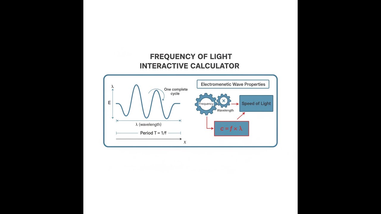
Electromagnetic Wave Diagram

Frequency of Light Calculator

Governing Equations

Theory & Practical Applications

Electromagnetic Wave Nature and the Wave-Particle Duality

Light exhibits a fundamental dual nature that manifests differently depending on the experimental context. The wave model, described by Maxwell's equations, treats light as oscillating electric and magnetic fields perpendicular to each other and to the direction of propagation. The frequency of these oscillations defines the color perceived by the human eye for visible wavelengths (approximately 430-770 THz) and determines energy content for all electromagnetic radiation. The particle model treats light as discrete packets of energy called photons, each carrying energy E = hf where h is Planck's constant.

A critical distinction often overlooked in basic treatments: while frequency remains invariant when light crosses material boundaries, wavelength decreases by the refractive index ratio. This has profound implications for optical resonator design. A Fabry-Pérot cavity resonant at 1550 nm in vacuum will support standing waves at λ/n = 1019 nm when filled with silicon (n = 3.48 at telecom wavelengths). Engineers designing integrated photonic circuits must account for this wavelength compression when calculating resonator dimensions, waveguide coupling distances, and distributed Bragg reflector periods.

Frequency-Dependent Phenomena in Real Systems

Dispersion—the frequency dependence of refractive index—limits performance in high-bandwidth optical communication systems. Standard single-mode fiber (SMF-28) exhibits chromatic dispersion of approximately 17 ps/(nm·km) at 1550 nm. For a 100 Gbps signal with spectral width Δλ ≈ 0.8 nm transmitted over 80 km, pulse spreading reaches Δt = 17 × 0.8 × 80 = 1088 ps. Since the bit period is only 10 ps (1/100 Gbps), severe intersymbol interference occurs unless dispersion compensation is implemented.

The frequency-dependent absorption coefficient α(f) determines penetration depth in materials. For biological tissue, near-infrared wavelengths (700-900 nm, corresponding to 330-428 THz) penetrate several centimeters due to minimal absorption by hemoglobin and water. This "optical window" enables non-invasive deep-tissue imaging and photobiomodulation therapy. Conversely, ultraviolet-C radiation (200-280 nm, 1071-1500 THz) penetrates only micrometers into human skin but effectively disrupts viral and bacterial DNA—the physical basis for UV-C germicidal lamps.

Worked Engineering Example: Laser Diode Specification

A telecommunications engineer must specify a laser diode for a dense wavelength division multiplexing (DWDM) system operating on the ITU-T G.694.1 grid. The system requires a channel centered at 193.1 THz with maximum frequency drift of ±1.25 GHz under temperature variations from 0°C to 70°C.

Part A: Calculate the center wavelength in vacuum

Using c = f × λ and solving for λ:

λ₀ = c / f = (2.99792458 × 10⁸ m/s) / (193.1 × 10¹² Hz) = 1.55234 × 10⁻⁶ m = 1552.34 nm

This wavelength falls in the C-band (1530-1565 nm), commonly used for long-haul fiber optic transmission.

Part B: Determine the allowable wavelength drift

The frequency drift tolerance is Δf = ±1.25 GHz = ±1.25 × 10⁹ Hz. We must find the corresponding wavelength tolerance. Taking the differential of c = fλ:

c = fλ → 0 = f(dλ) + λ(df) → dλ/df = -λ/f

For small variations: Δλ ≈ -(λ/f) × Δf

Δλ = -(1.55234 × 10⁻⁶ m / 193.1 × 10¹² Hz) × (±1.25 × 10⁹ Hz) = ∓1.004 × 10⁻¹¹ m = ∓0.01004 nm

The allowable wavelength drift is ±0.010 nm (±10 pm). Note the negative sign indicates frequency and wavelength vary inversely.

Part C: Calculate photon energy and required output power

For quantum efficiency calculations, determine the photon energy:

E = hf = (6.62607015 × 10⁻³⁴ J·s) × (193.1 × 10¹² Hz) = 1.2793 × 10⁻¹⁹ J

Converting to electronvolts: E = (1.2793 × 10⁻¹⁹ J) / (1.602176634 × 10⁻¹⁹ J/eV) = 0.7985 eV

If the system requires 10 mW optical output power, calculate the photon emission rate:

Power = (number of photons/second) × (energy per photon)

Photon rate = P / E = (10 × 10⁻³ W) / (1.2793 × 10⁻¹⁹ J) = 7.82 × 10¹⁶ photons/second

This enormous photon flux (78.2 petaphotons/second) illustrates why classical wave descriptions suffice for most macroscopic optical systems—quantum discreteness becomes negligible when dealing with such large photon numbers.

Part D: Wavelength in fiber core

The fiber core has refractive index n = 1.4682 at 1552.34 nm. Calculate the wavelength inside the fiber:

λ_fiber = λ₀ / n = 1552.34 nm / 1.4682 = 1057.05 nm

This 32% wavelength reduction affects guided-wave phenomena such as modal cutoff wavelengths and effective mode field diameter. For a fiber with V-number calculated using vacuum wavelength, the actual guided mode experiences the compressed wavelength, affecting coupling efficiency to integrated photonic devices.

Applications Across Industries

Optical Communications: The 1550 nm wavelength (193.1 THz) serves as the primary carrier for global fiber optic networks due to minimal attenuation (0.2 dB/km) and compatibility with erbium-doped fiber amplifiers (EDFAs). System designers exploit the 1530-1565 nm C-band and 1565-1625 nm L-band to create 80+ DWDM channels spaced 50 GHz (0.4 nm) apart, achieving aggregate capacities exceeding 10 Tbps on a single fiber pair.

Medical Phototherapy: Light-tissue interactions are strongly frequency dependent. Blue light at 463 nm (648 THz) treats neonatal jaundice by photoisomerizing bilirubin. Red light at 660 nm (454 THz) and near-infrared at 850 nm (353 THz) penetrate 2-3 cm into tissue, stimulating mitochondrial cytochrome c oxidase and modulating cellular metabolism through photobiomodulation mechanisms still under investigation.

Semiconductor Manufacturing: Extreme ultraviolet lithography (EUVL) at 13.5 nm (22.2 PHz) enables <7 nm process nodes by reducing diffraction-limited feature sizes. The photon energy at this wavelength is 91.8 eV—sufficient to directly break chemical bonds in photoresists without requiring multi-photon processes. However, essentially all materials absorb strongly at this frequency, necessitating reflective optics with multilayer Mo/Si coatings and operation in high vacuum.

Spectroscopic Analysis: Atomic emission and absorption spectroscopy relies on characteristic frequencies corresponding to electronic transitions. The sodium D-line doublet at 589.0 nm and 589.6 nm (508.8 and 508.3 THz) arises from the 3²P₃/₂,₁/₂ → 3²S₁/₂ transitions. Frequency precision better than 1 MHz enables laser cooling of sodium atoms to microkelvin temperatures for quantum computing applications.

Radio Astronomy: The 21-cm hydrogen line at 1420.4 MHz arises from the hyperfine transition in neutral atomic hydrogen. This specific frequency allows astronomers to map galactic hydrogen distribution and measure cosmological redshifts. The corresponding photon energy (5.87 μeV) is far too small for chemical effects but perfectly suited for large-scale coherent detection with radio interferometry arrays.

Non-Ideal Behaviors and Engineering Limitations

Real electromagnetic sources exhibit finite spectral linewidth Δf due to fundamental and technical noise processes. For laser diodes, spontaneous emission contributes a Lorentzian linewidth component following the Schawlow-Townes formula, modified by the linewidth enhancement factor α. A typical 1550 nm distributed feedback (DFB) laser with 30 mW output has intrinsic linewidth ~100 kHz, but thermal fluctuations and injection current noise increase practical linewidth to 1-10 MHz unless active stabilization is employed.

The group velocity (dω/dk) differs from phase velocity (ω/k) in dispersive media, causing pulse envelope and carrier to propagate at different speeds. In optical fiber, second-order dispersion β₂ = d²k/dω² causes Gaussian pulses to broaden as √(1 + (z/L_D)²) where L_D = T₀²/|β₂| is the dispersion length and T₀ is the initial pulse width. For T₀ = 10 ps in standard fiber (β₂ ≈ -20 ps²/km at 1550 nm), dispersion length is merely 5 km—after which pulse broadening becomes significant.

For additional wave and optics calculations, explore the complete engineering calculator library.

Frequently Asked Questions