Designing a resonant system — whether an RF filter, optical cavity, or communication channel — means knowing exactly where your signal lives in the frequency domain. Use this Frequency Bandwidth Interactive Calculator to calculate center frequency, bandwidth, quality factor (Q-factor), and upper and lower cutoff frequencies using any 2 of those parameters as inputs. Getting these numbers right is non-negotiable in RF circuit design, telecommunications infrastructure, audio engineering, and optical resonator work. This page covers the key equations, a worked example, full theory, and an FAQ.
What is Frequency Bandwidth?
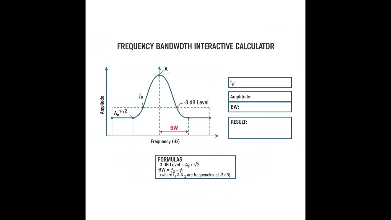
Frequency bandwidth is the range of frequencies over which a system — a filter, antenna, resonator, or channel — operates effectively. It's the gap between the upper and lower cutoff frequencies where signal power stays above half its peak value.
Simple Explanation
Think of it like a window. Your system only lets through sounds (or signals) within a certain frequency range — that range is the bandwidth. A narrow window is selective but misses a lot; a wide window lets through more but is less focused. The center frequency is the middle of that window, and the Q-factor tells you how narrow or wide the window is relative to where it sits.
📐 Browse all 1000+ Interactive Calculators
Bandwidth Diagram

Frequency Bandwidth Calculator
How to Use This Calculator
- Select your calculation mode from the dropdown — choose which parameter you want to solve for (Bandwidth, Q-factor, Center Frequency, Lower Cutoff, or Upper Cutoff).
- Enter the lower cutoff frequency (fL) or center frequency (f₀) in Hz, depending on the selected mode.
- Enter the upper cutoff frequency (fH) or bandwidth (BW) in Hz, depending on the selected mode.
- Click Calculate to see your result.
Frequency Bandwidth Interactive Visualizer
Visualize how center frequency, bandwidth, and quality factor interact in resonant systems. Watch the frequency response curve update as you adjust parameters to understand RF filters, communication channels, and optical resonators.
BANDWIDTH
100 Hz
LOWER CUTOFF
950 Hz
UPPER CUTOFF
1050 Hz
FRAC. BW
10.0%
FIRGELLI Automations — Interactive Engineering Calculators
Key Equations
Use the formula below to calculate frequency bandwidth and related resonant system parameters.
where BW is the bandwidth (Hz), fH is the upper cutoff frequency (Hz), and fL is the lower cutoff frequency (Hz).
where f₀ is the center frequency (Hz). This geometric mean applies to systems with symmetrical frequency response on a logarithmic scale.
where Q is the dimensionless quality factor, representing the ratio of energy stored to energy dissipated per cycle in resonant systems.
where FBW is the fractional bandwidth (dimensionless or expressed as percentage), inversely related to quality factor.
These exact expressions account for the asymmetry of cutoff frequencies about the center frequency in resonant systems.
Simple Example
A bandpass filter has a lower cutoff of 900 Hz and an upper cutoff of 1,100 Hz.
- BW = 1,100 − 900 = 200 Hz
- f₀ = √(900 × 1,100) = 994.99 Hz
- Q = 994.99 / 200 = 4.97
- Fractional Bandwidth = 200 / 994.99 = 20.1%
Theory & Practical Applications
Fundamental Physics of Frequency Bandwidth
Frequency bandwidth quantifies the range of frequencies over which a system effectively transmits, resonates, or responds to oscillatory input. In resonant systems—from mechanical oscillators to electromagnetic cavities—the bandwidth defines the frequency interval where the response amplitude exceeds 1/√2 (approximately 70.7%) of its peak value, corresponding to the half-power points or -3 dB levels. This definition arises naturally from energy considerations: at the cutoff frequencies, the power transmitted or stored drops to half its maximum value, representing the boundary between efficient and inefficient operation.
The center frequency f₀ represents the resonant frequency where maximum response occurs. For narrowband systems where BW ≪ f₀, the arithmetic mean (fL + fH)/2 approximates f₀. However, the rigorous definition uses the geometric mean f₀ = √(fL×fH), which ensures symmetry on logarithmic frequency scales and accurately reflects the physics of coupled oscillators, LC circuits, and optical resonators. This distinction becomes critical for wideband systems: a filter centered at 1 GHz with 500 MHz bandwidth has an arithmetic center of 1 GHz but a geometric center of approximately 968 MHz, affecting impedance matching and phase response.
Quality Factor and Energy Dissipation
The quality factor Q = f₀/BW is perhaps the most important dimensionless parameter characterizing resonant systems. Physically, Q represents the ratio of energy stored per cycle to energy dissipated per radian, or equivalently, 2π times the ratio of stored energy to energy loss per cycle. High-Q systems (Q greater than 100) exhibit sharp resonance peaks with narrow bandwidths, allowing precise frequency selection but slow transient response. Low-Q systems (Q less than 10) sacrifice selectivity for broader bandwidth and faster settling times.
In electrical circuits, Q is limited by resistive losses in inductors and capacitors. A practical LC bandpass filter with Q = 50 achieves 2% fractional bandwidth, suitable for single-channel radio reception. Mechanical resonators like quartz crystals exploit minimal internal friction to reach Q values exceeding 10,000, enabling frequency references with parts-per-million stability. Optical cavities in laser systems can achieve Q greater than 10⁸ through mirror reflectivities above 99.999%, confining photons for thousands of round trips and producing coherent light with sub-kHz linewidths from cavity dimensions measured in centimeters.
Bandwidth in Communication Systems
In telecommunications, bandwidth directly determines information capacity through the Shannon-Hartley theorem: C = BW × log₂(1 + SNR), where C is channel capacity in bits per second and SNR is the signal-to-noise ratio. A 4G LTE channel with 20 MHz bandwidth and 20 dB SNR theoretically supports 133 Mbps, though practical protocols achieve 60-70% of this limit due to coding overhead and guard bands. The relationship between bandwidth and data rate explains the telecommunications industry's relentless pursuit of higher-frequency spectrum: millimeter-wave 5G systems operating at 28 GHz can allocate contiguous 400 MHz channels impossible at crowded sub-6 GHz frequencies.
Filter design in communication systems requires careful bandwidth specification to pass desired signals while rejecting adjacent channels. A superheterodyne receiver downconverts a 2.4 GHz WiFi signal to a 100 MHz intermediate frequency, where a crystal filter with ±10 MHz bandwidth isolates the channel. The rolloff steepness—how rapidly attenuation increases outside the passband—depends on filter order: each additional pole in a Butterworth filter adds 20 dB/decade rejection, but also increases group delay variation, potentially causing inter-symbol interference in digital modulation.
Optical Bandwidth and Spectral Linewidth
In optics, bandwidth takes on wavelength-dependent character due to the relationship c = fλ. Differentiating yields Δλ/λ = -Δf/f, connecting wavelength bandwidth to frequency bandwidth. A laser operating at λ = 1550 nm (f = 193.5 THz) with 100 GHz linewidth corresponds to Δλ ≈ 0.8 nm. Optical engineers often work in wavelength units for convenience, but frequency bandwidth governs the fundamental physics of mode spacing in cavities and chromatic dispersion in fibers.
Fourier transform relationships impose fundamental limits: Δf × Δt ≥ 1/(4π), where Δt is the pulse duration. A 100 femtosecond laser pulse necessarily has spectral bandwidth exceeding 4.4 THz (35 nm at 800 nm wavelength), explaining why ultrafast lasers require broadband gain media like Ti:sapphire. This time-bandwidth product governs spectroscopy resolution: measuring the 21 cm hydrogen line (1420 MHz) to 1 kHz precision requires integration times exceeding 1 millisecond, fundamentally limiting radioastronomy observation rates.
Worked Example: RF Cavity Design for Particle Accelerator
Problem: Design the bandwidth specifications for a 1.3 GHz superconducting radio-frequency (SRF) cavity intended for a linear particle accelerator. The cavity must accelerate electron bunches spaced 714 ns apart (corresponding to 1.4 MHz bunch repetition rate) while maintaining sufficient loaded quality factor to reduce required RF power. The unloaded cavity Q₀ = 2°10¹⁰ is fixed by superconductor properties. Calculate: (a) the optimal loaded Q_L to achieve 1.8 MHz bandwidth for beam loading compensation, (b) the resulting cutoff frequencies, (c) the coupling coefficient β required to achieve this loaded Q, and (d) the power overhead factor compared to critically coupled operation.
Solution:
Part (a): The loaded quality factor relates directly to bandwidth through Q_L = f₀/BW. Given f₀ = 1.3 GHz and target BW = 1.8 MHz:
Q_L = f₀ / BW = (1.3 × 10⁹ Hz) / (1.8 × 10⁶ Hz) = 722.2
This loaded Q is dramatically lower than the unloaded Q₀, indicating heavy coupling to external waveguides—essential for extracting power to the beam while accommodating frequency variations from mechanical vibrations and helium pressure fluctuations in the cryogenic system.
Part (b): Using the exact cutoff frequency formulas:
Term = BW/(2f₀) = (1.8×10⁶)/(2×1.3×10⁹) = 6.923×10⁻⁴
Discriminant = (6.923×10⁻⁴)² + 1 = 1.0000004793
√(Discriminant) = 1.00000024
f_L = f₀[√(1 + (BW/2f₀)²) - BW/2f₀]
f_L = 1.3×10⁹ × [1.00000024 - 6.923×10⁻⁴]
f_L = 1.3×10⁹ × 0.9993081 = 1,299,100,530 Hz ≈ 1.2991 GHz
f_H = f₀[√(1 + (BW/2f₀)²) + BW/2f₀]
f_H = 1.3×10⁹ × [1.00000024 + 6.923×10⁻⁴]
f_H = 1.3×10⁹ × 1.0006925 = 1,300,900,250 Hz ≈ 1.3009 GHz
Verification: BW = f_H - f_L = 1,300,900,250 - 1,299,100,530 = 1,799,720 Hz ≈ 1.8 MHz ✓
Part (c): The coupling coefficient β relates unloaded and loaded quality factors through:
1/Q_L = 1/Q₀ + 1/Q_ext
where Q_ext is the external quality factor determined by coupling. Solving for Q_ext:
1/Q_ext = 1/Q_L - 1/Q₀ = 1/722.2 - 1/(2×10¹⁰)
1/Q_ext = 0.001385 - 0.00000000005 ≈ 0.001385
Q_ext = 722.2
The coupling coefficient β = Q₀/Q_ext:
β = (2×10¹⁰) / 722.2 = 2.77×10⁷
This enormous coupling coefficient indicates severe overcoupling—the cavity is coupled so strongly to the external circuit that Q_L ≈ Q_ext, with the intrinsic Q₀ having negligible effect. This regime is standard for accelerator cavities where beam loading extracts megawatts of RF power.
Part (d): Critical coupling occurs when β = 1 (Q_ext = Q₀), maximizing power transfer efficiency at a single frequency. For our overcoupled case, the reflection coefficient at resonance is:
Γ = (β - 1)/(β + 1) = (2.77×10⁷ - 1)/(2.77×10⁷ + 1) ≈ 0.99999993
This means 99.99999% of incident power reflects at the cavity resonance—seemingly catastrophic. However, the power absorbed is:
P_absorbed/P_incident = 4β/(β+1)² = 4×2.77×10⁷/(2.77×10⁷+1)² ≈ 1.44×10⁻⁷
The power overhead factor compared to critical coupling (where all incident power is absorbed) is:
Overhead = 1/(P_absorbed/P_incident) = (β+1)²/(4β) ≈ 6.9×10⁶
This factor appears to demand 6.9 million times more RF power, but the physics is subtle: the high Q₀ stores enormous energy, so even this tiny fraction of absorbed power maintains the accelerating gradient. The real limitation is that the klystron must produce enough power to overcome the reflected wave interference pattern and charge the cavity to operating voltage during the fill time —_fill ≈ Q_L/πf₀ = 177 microseconds—far longer than the 714 ns bunch spacing, explaining why accelerator cavities run continuously rather than pulsing for each bunch.
Industrial Applications Across Domains
Wireless Communication Infrastructure: Cellular base stations employ cavity filters with Q factors between 5,000 and 10,000 to isolate transmit and receive bands separated by as little as 45 MHz at 1.9 GHz (2.4% fractional bandwidth). These filters must handle kilowatts of transmit power while providing 100+ dB isolation to prevent receiver desensitization, requiring silver-plated copper cavities with precision-tuned irises and computer-controlled thermal compensation to maintain alignment over temperature variations.
Medical Imaging: Magnetic resonance imaging (MRI) systems operate at the Larmor frequency f₀ = γB₀, where γ is the gyromagnetic ratio and B₀ is the main magnetic field strength. A 3 Tesla clinical scanner uses 128 MHz for hydrogen imaging, with RF coils designed for Q = 100-200 to maximize SNR while maintaining sufficient bandwidth (0.6-1.3 MHz) to accommodate the chemical shift range of different tissue types and rapid gradient switching during echo-planar imaging sequences.
Atomic Timekeeping: Chip-scale atomic clocks (CSACs) interrogate the 87Rb ground-state hyperfine transition at 6.834 GHz with a 100 Hz interrogation bandwidth, yielding Q = 6.8×10⁷. The fractional frequency stability approaches 10⁻¹¹ after 1-day integration, enabling GPS-free navigation in environments where satellite signals are denied. The narrow bandwidth imposes strict requirements on local oscillator phase noise and temperature stability of the vapor cell.
Vibration Isolation: Seismic isolation systems for gravitational wave detectors like LIGO employ mechanical resonators with Q factors exceeding 10⁶ at oscillation frequencies near 1 Hz, achieved through fused silica fibers supporting 40 kg mirrors. The sub-millihertz bandwidth enables attenuation of ground motion by factors exceeding 10⁹ at the 100 Hz gravitational wave detection band, crucial for observing binary black hole mergers at cosmological distances.
Bandwidth-Delay Product and Causality
A subtle but fundamental constraint connects bandwidth to transient response through the Kramers-Kronig relations, which enforce causality in linear systems. A filter with bandwidth BW requires minimum settling time Δt ≈ 1/BW to respond to a step input, independent of filter topology. This manifests practically in tracking receivers: a GPS receiver with 2 MHz bandwidth requires ≥0.5 microseconds to lock onto a satellite signal after acquisition, fundamentally limiting how quickly a receiver can switch between satellites during high-dynamics maneuvers.
The bandwidth-delay product also appears in optical fiber communications through chromatic dispersion. A single-mode fiber with dispersion parameter D = 17 ps/(nm·km) limits the product of bit rate and transmission distance: BW × L less than approximately 10⁴ GHz·km before pulse spreading causes inter-symbol interference. A 10 Gbps signal (10 GHz bandwidth) can propagate 1000 km before requiring dispersion compensation through fiber Bragg gratings or digital signal processing—constraints that shaped the architecture of transoceanic fiber networks.
Frequently Asked Questions
Free Engineering Calculators
Explore our complete library of free engineering and physics calculators.
Browse All Calculators →🔗 Explore More Free Engineering Calculators
About the Author
Robbie Dickson — Chief Engineer & Founder, FIRGELLI Automations
Robbie Dickson brings over two decades of engineering expertise to FIRGELLI Automations. With a distinguished career at Rolls-Royce, BMW, and Ford, he has deep expertise in mechanical systems, actuator technology, and precision engineering.
Need to implement these calculations?
Explore the precision-engineered motion control solutions used by top engineers.


