Darcys Law Interactive Calculator

Darcy's Law describes the flow of fluid through porous media and forms the foundation of groundwater hydrology, petroleum engineering, and filtration design. This interactive calculator solves for discharge rate, hydraulic conductivity, cross-sectional area, or hydraulic gradient across multiple engineering scenarios including groundwater wells, soil permeability testing, and industrial filtration systems.

📐 Browse all free engineering calculators

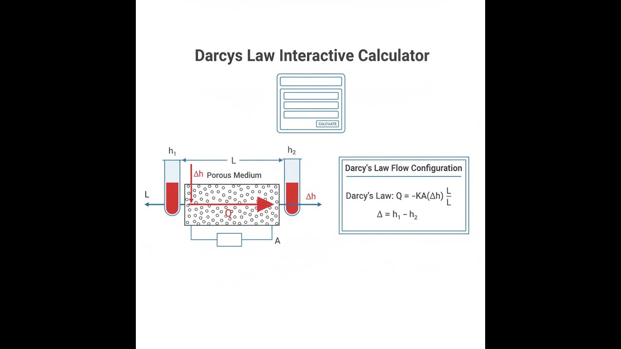
Visual Diagram

Interactive Calculator

Governing Equations

Theory & Practical Applications

Fundamental Physics of Darcy's Law

Darcy's Law, established by Henry Darcy in 1856 during his investigation of water flow through sand filters in Dijon, France, remains the cornerstone equation for describing fluid flow through porous media. The law applies specifically to laminar flow conditions where viscous forces dominate over inertial forces, typically characterized by Reynolds numbers below 1-10 in porous media. Unlike pipe flow where Reynolds number is based on pipe diameter, porous media Reynolds numbers use characteristic grain size (typically d₁₀) as the length scale: Re = ρvd₁₀/μ, where ρ is fluid density, v is Darcy velocity, and μ is dynamic viscosity.

The hydraulic conductivity K represents the ease with which fluid moves through the porous matrix and depends on both medium properties (permeability, porosity, grain size distribution, tortuosity) and fluid properties (density and viscosity). The intrinsic permeability k (measured in m² or darcys, where 1 darcy ≈ 9.87×10⁻¹³ m²) separates these dependencies: K = kρg/μ. For water at 20°C (μ ≈ 1.002×10⁻³ Pa·s, ρ = 998 kg/m³), this relationship allows conversion between hydraulic conductivity and intrinsic permeability. A sand with k = 1×10⁻¹¹ m² has K ≈ 1×10⁻⁴ m/s for water, but only K ≈ 1.3×10⁻⁷ m/s for crude oil with viscosity 100 times greater.

Critical Engineering Limitations and Non-Darcy Flow

Darcy's Law assumes linear proportionality between hydraulic gradient and discharge velocity, valid only under laminar conditions. When flow velocities increase sufficiently that inertial forces become significant, the Forchheimer equation applies: i = (μ/kρg)v + (β/g)v², where β is the non-Darcy coefficient (m⁻¹). This quadratic term becomes significant at Reynolds numbers above 10, common in coarse gravels, near high-capacity pumping wells, or in fractured rock where preferential flow paths create locally high velocities. Engineers must verify Re < 1 for fine sands, Re < 10 for medium sands before applying Darcy's Law, otherwise predicted flow rates can exceed actual performance by 15-40% in transitional regimes.

Another critical limitation involves heterogeneity and anisotropy. Natural geological formations rarely exhibit uniform hydraulic conductivity; K can vary by 2-3 orders of magnitude across stratified deposits. Horizontal conductivity (K_h) typically exceeds vertical conductivity (K_v) by factors of 3-100 in sedimentary deposits due to preferential layering. Three-dimensional flow analysis requires the full conductivity tensor, and equivalent conductivities for layered systems follow: K_eq,parallel = Σ(K_ib_i)/Σb_i for parallel flow, and 1/K_eq,series = Σ(b_i/K_i)/Σb_i for perpendicular flow, where b_i represents layer thickness.

Groundwater Engineering Applications

In well hydraulics, Darcy's Law forms the basis for predicting sustainable yield and drawdown patterns. For a fully penetrating well in a confined aquifer, combining Darcy's Law with radial flow geometry yields the Thiem equation: Q = 2πKb(h₁-h₂)/ln(r₁/r₂), where b is aquifer thickness, and h₁, h₂ are heads at radial distances r₁, r₂. Municipal water supply wells typically operate with specific capacities (Q/Δh) of 10-50 L/s/m in productive aquifers. A 200 mm diameter well screened across 15 m of confined sand with K = 2.5×10⁻⁴ m/s can theoretically produce 12-18 L/s with 3-5 m of drawdown at the well face, though actual performance depends critically on well construction efficiency (skin factor) and aquifer boundary conditions.

Contaminant transport modeling requires Darcy velocity as the advective component. The actual groundwater seepage velocity v_s = v/n_e, where n_e is effective porosity (typically 0.25-0.35 for sands, 0.01-0.05 for clays). A contaminant plume in sand with hydraulic gradient i = 0.003, K = 5×10⁻⁵ m/s, and n_e = 0.28 travels at v_s = (5×10⁻⁵ × 0.003)/0.28 ≈ 5.4×10⁻⁷ m/s = 1.7 cm/day = 6.2 m/year. However, dispersion and retardation (sorption) significantly modify actual plume migration, requiring coupled advection-dispersion equations for accurate prediction.

Geotechnical and Foundation Engineering

Seepage beneath hydraulic structures creates uplift pressures that reduce effective stress and compromise stability. Sheet pile cofferdams, concrete dams, and levees require seepage analysis via flow nets or finite element methods applying Darcy's Law at each node. The critical hydraulic gradient i_cr for cohesionless soils equals (G_s-1)/(1+e), where G_s is specific gravity (≈2.65 for quartz) and e is void ratio. For loose sand with e = 0.7, i_cr ≈ 0.97; actual design exit gradients must remain below 0.25-0.5 times i_cr to prevent piping failure, requiring factors of safety of 2-4.

Consolidation of saturated clays under structural loads follows from Darcy's Law coupled with soil compressibility. Terzaghi's one-dimensional consolidation equation c_v = K/(γ_wm_v) relates consolidation coefficient c_v to hydraulic conductivity K and volume compressibility m_v. For soft clay with K = 1×10⁻⁹ m/s and m_v = 3×10⁻⁴ m²/kN, c_v ≈ 0.34 m²/year. A 4 m thick clay layer beneath a building foundation requires approximately t₉₀ = (0.848 × H²)/c_v = 40 years to reach 90% primary consolidation, necessitating surcharge preloading or vertical drain systems to accelerate settlement and enable construction.

Industrial Filtration and Petroleum Engineering

Industrial sand filters, membrane systems, and packed bed reactors operate on Darcy flow principles. Clean bed head loss predictions use the Kozeny-Carman equation derived from Darcy's Law: Δh/L = 150μv(1-n)²/(ρgd²n³), where d is mean grain diameter and n is porosity. A rapid sand filter (d = 0.6 mm, n = 0.42) operating at v = 5 m/h (1.39×10⁻³ m/s) develops clean bed head loss of 0.12 m/m, increasing to 1.5-2.5 m/m at terminal head loss when particulate accumulation reduces effective porosity to 0.32-0.35. Backwash cycles restore permeability, with optimal timing based on head loss monitoring rather than fixed schedules.

Petroleum reservoir engineering applies Darcy's Law to predict oil and gas production from porous reservoir rock. Multi-phase flow modifications account for relative permeabilities k_r,oil and k_r,water (both ≤ 1, sum < 1) that depend on saturation history. A sandstone reservoir with k = 200 millidarcys (2×10⁻¹³ m²), 30% porosity, and 100 m pay zone thickness exhibits initial productivity indices of 5-15 m³/day/bar under primary recovery. Enhanced oil recovery techniques (waterflooding, gas injection, chemical flooding) modify relative permeability curves and effective viscosity, requiring iterative numerical simulation coupling Darcy's Law with phase behavior models to optimize production strategy and forecast ultimate recovery factors of 35-60% of original oil in place.

Worked Example: Municipal Well Field Design

Problem: A municipality needs to design a well field in a confined sand aquifer to supply 450 m³/day (5.21 L/s) for a new residential development. Site investigation reveals the aquifer has the following properties: saturated thickness b = 18.5 m, horizontal hydraulic conductivity K_h = 3.4×10⁻⁴ m/s, vertical hydraulic conductivity K_v = 8.2×10⁻⁵ m/s, regional hydraulic gradient i₀ = 0.0018 (to the east), porosity n = 0.34, and effective porosity n_e = 0.29. The wellfield will consist of two wells spaced 85 m apart, each screened across the full aquifer thickness with 250 mm diameter screens.

Part A: Calculate the natural (undisturbed) groundwater discharge per unit width through the aquifer cross-section perpendicular to flow.

Part B: Determine the required drawdown at each well to achieve the target combined discharge of 450 m³/day, assuming both wells operate identically.

Part C: Calculate the natural seepage velocity and estimate time for a conservative tracer released 500 m upgradient to reach the well field.

Part D: Assess whether flow conditions satisfy Darcy's Law assumptions.

Solution Part A: For natural regional flow, apply Darcy's Law with the horizontal conductivity. Considering a 1 m wide cross-section perpendicular to flow:

Q_natural = K_h × A × i₀
A = b × (unit width) = 18.5 m × 1 m = 18.5 m²
Q_natural = (3.4×10⁻⁴ m/s) × (18.5 m²) × (0.0018)
Q_natural = 1.132×10⁻⁵ m³/s = 0.01132 L/s per meter width
Q_natural = 978 m³/day per meter width

This represents the natural through-flow capacity of the aquifer, which is substantial relative to the proposed pumping rate.

Solution Part B: For a fully penetrating well in a confined aquifer with radius of influence R and drawdown s at the well face (radius r_w = 0.125 m for 250 mm screen), the Thiem equation modified from radial Darcy flow gives:

Q_well = (2πKb × s) / ln(R/r_w)

Each well must produce Q_well = 450/(2 × 86400) = 2.604×10⁻³ m³/s. Assuming radius of influence R ≈ 300 m (typical for confined aquifer pumping tests, verified through type curve analysis):

2.604×10⁻³ = (2π × 3.4×10⁻⁴ × 18.5 × s) / ln(300/0.125)
2.604×10⁻³ = (0.03952 × s) / 7.886
2.604×10⁻³ = 0.005012 × s
s = 0.519 m

Required drawdown at each well face is approximately 0.52 m, which is quite modest (only 2.8% of aquifer thickness), indicating sustainable operation well within aquifer capacity. However, well interference must be checked since wells are only 85 m apart. Using principle of superposition, the total drawdown at Well 1 includes drawdown from its own pumping plus drawdown induced by Well 2 pumping 85 m away:

s_additional = Q_well × ln(R/r_separation) / (2πKb)
s_additional = 2.604×10⁻³ × ln(300/85) / (2π × 3.4×10⁻⁴ × 18.5)
s_additional = 2.604×10⁻³ × 1.258 / 0.03952
s_additional = 0.083 m

Total drawdown at each well = 0.519 + 0.083 = 0.602 m, still acceptably low.

Solution Part C: Natural seepage velocity (actual pore velocity) determines conservative tracer migration:

Darcy velocity: v = K_h × i₀ = 3.4×10⁻⁴ × 0.0018 = 6.12×10⁻⁷ m/s
Seepage velocity: v_s = v / n_e = 6.12×10⁻⁷ / 0.29 = 2.11×10⁻⁶ m/s
v_s = 0.182 m/day = 66.5 m/year

Travel time over 500 m distance (assuming purely advective transport):

t = distance / v_s = 500 m / (2.11×10⁻⁶ m/s)
t = 2.37×10⁸ seconds = 2740 days = 7.5 years

Actual breakthrough would occur earlier due to hydrodynamic dispersion and slightly faster due to well capture zone acceleration of flow, but this provides conservative estimate for wellhead protection zone delineation.

Solution Part D: Verify Darcy's Law validity by calculating Reynolds number near the well face where velocity is highest:

Maximum Darcy velocity (radial flow at well screen): v_max = Q_well / (2πr_wb)
v_max = 2.604×10⁻³ / (2π × 0.125 × 18.5) = 1.792×10⁻⁴ m/s

Using characteristic grain size d₁₀ ≈ 0.15 mm (typical for medium sand) and water properties at 15°C (ρ = 999 kg/m³, μ = 1.14×10⁻³ Pa·s):

Re = ρ × v_max × d₁₀ / μ
Re = (999 × 1.792×10⁻⁴ × 0.00015) / 1.14×10⁻³
Re = 0.0236

Since Re < 1, flow remains firmly in the laminar regime where Darcy's Law is valid, even immediately adjacent to the well screen where velocities are maximum. The design is hydraulically sound.

Frequently Asked Questions