Knowing your inventory turnover ratio is one thing — knowing what to do about it is another. When cash is tied up in slow-moving stock, every day of delay has a real cost in working capital, storage, and obsolescence risk. Use this Inventory Turnover COGS Calculator to calculate your turnover ratio, Days Inventory Outstanding (DIO), optimal inventory level, and required COGS using your actual cost of goods sold and average inventory figures. It matters across manufacturing, distribution, and retail — anywhere that inventory velocity directly affects cash flow and operational efficiency. This page covers the core formulas, a worked example, theory behind COGS-based turnover, and a FAQ section.
What is Inventory Turnover?
Inventory turnover is a measure of how many times a business sells and replaces its stock over a given period. A higher number means inventory is moving fast — a lower number means capital is sitting on shelves longer than it should be.
Simple Explanation
Think of inventory turnover like a shelf at a grocery store. If a product sells out and gets restocked 6 times in a year, it has a turnover of 6. The faster the shelf clears, the less money is stuck waiting to become a sale. Slow-moving inventory is just cash you can't spend yet.
📐 Browse all 1000+ Interactive Calculators
Table of Contents
How to Use This Calculator
- Select your calculation mode from the dropdown — choose what you want to solve for (turnover ratio, required COGS, optimal inventory, etc.).
- Enter your Cost of Goods Sold (COGS) — the annual total cost of products sold, in currency units.
- Enter your Average Inventory value — typically (Beginning Inventory + Ending Inventory) ÷ 2.
- Click Calculate to see your result.
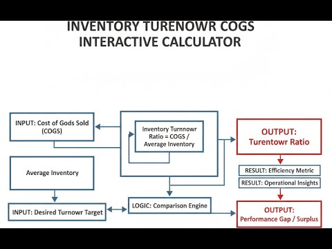
Visual Diagram

Inventory Turnover Calculator
Inventory Turnover COGS Interactive Visualizer
Watch how Cost of Goods Sold and average inventory values affect your turnover ratio, days inventory outstanding, and cash flow efficiency. Adjust inputs to see real-time impacts on working capital and operational performance.
TURNOVER RATIO
6.0x
DAYS OUTSTANDING
60.8 days
DAILY COGS
$1,644
FIRGELLI Automations — Interactive Engineering Calculators
Core Equations
Use the formula below to calculate inventory turnover ratio.
Inventory Turnover Ratio
Turnover = COGS / Average Inventory
Where:
• COGS = Cost of Goods Sold for the period (currency units)
• Average Inventory = (Beginning Inventory + Ending Inventory) / 2 (currency units)
• Turnover = Number of times inventory is sold and replaced (dimensionless)
Use the formula below to calculate Days Inventory Outstanding.
Days Inventory Outstanding (DIO)
DIO = Period (days) / Turnover Ratio
Alternatively:
DIO = (Average Inventory / COGS) × Period (days)
Where:
• DIO = Days Inventory Outstanding (days)
• Period = Analysis period, typically 365 days for annual calculations
Use the formula below to calculate required inventory for a target turnover.
Required Inventory for Target Turnover
Average Inventory = COGS / Target Turnover
Where:
• Average Inventory = Required average inventory value (currency units)
• Target Turnover = Desired turnover ratio (times per period)
Use the formula below to calculate the COGS required to hit a target turnover.
Required COGS for Target Turnover
COGS = Target Turnover × Average Inventory
Where:
• COGS = Required Cost of Goods Sold to achieve target (currency units)
• This equation determines sales volume needed for desired inventory efficiency
Simple Example
A distributor has annual COGS of $600,000 and average inventory of $100,000.
- Turnover = $600,000 / $100,000 = 6.0x
- DIO = 365 / 6.0 = 60.8 days
- To hit 8x turnover: required inventory = $600,000 / 8 = $75,000
Theory & Engineering Applications
Inventory turnover ratio using Cost of Goods Sold represents one of the most powerful operational metrics in manufacturing, distribution, and retail management. Unlike revenue-based turnover calculations, COGS-based turnover provides a more accurate picture of physical inventory movement because it measures the actual cost of products sold rather than inflated sales prices. This metric directly links financial performance to operational efficiency, revealing how effectively a company converts inventory investments into sales and ultimately cash flow.
Fundamental Theory and Financial Mechanics
The inventory turnover ratio quantifies the number of times a company sells and replaces its entire inventory during a specific period, typically one year. The formula divides annual COGS by average inventory value, where average inventory is calculated as the mean of beginning and ending inventory for the period. This metric serves as a velocity indicator—higher turnover means inventory moves faster through the supply chain, reducing holding costs, obsolescence risk, and working capital requirements. A turnover ratio of 6.0, for example, indicates inventory is completely replaced six times annually, or approximately every 61 days.
The relationship between turnover and Days Inventory Outstanding (DIO) provides complementary perspectives on the same phenomenon. While turnover ratio expresses frequency, DIO converts this to a time-based metric showing how many days of sales current inventory can support. The mathematical relationship DIO = 365 / Turnover creates an inverse proportionality: doubling turnover from 4 to 8 cuts DIO from 91 to 46 days. This duality allows managers to think in terms of either rotation frequency or time coverage, depending on which perspective best suits their decision-making context.
A critical but often overlooked aspect of COGS-based turnover is its sensitivity to inventory valuation methods. Companies using FIFO (First-In-First-Out) during inflationary periods report lower COGS and higher ending inventory values compared to LIFO (Last-In-First-Out) users, resulting in different turnover ratios for operationally identical businesses. Similarly, the inclusion or exclusion of overhead costs in inventory valuation—absorption costing versus variable costing—can shift turnover ratios by 15-30% without any change in physical inventory management. These accounting nuances mean that turnover ratios should be compared only within consistent valuation frameworks and interpreted alongside other operational metrics like stockout frequency and order fulfillment rates.
Industry Benchmarks and Performance Standards
Optimal inventory turnover varies dramatically across industries based on product perishability, value density, supply chain complexity, and demand volatility. Grocery retailers typically achieve 12-15 turns annually due to perishable goods and high-volume, low-margin models. Fast-fashion retailers like Zara target 10-12 turns to minimize fashion obsolescence. In contrast, heavy equipment manufacturers may operate efficiently at 3-4 turns given long production cycles and high unit values. Aerospace manufacturers working on multi-year contracts often maintain turnover ratios below 2.0, where inventory represents work-in-progress on complex assemblies rather than finished goods awaiting sale.
The pharmaceutical industry presents an interesting case study in turnover optimization under regulatory constraints. While raw materials and packaging might turn 8-10 times annually, finished pharmaceuticals often turn only 3-5 times due to extensive quality testing, batch tracking requirements, and safety stock regulations. Companies must balance the financial pressure to reduce inventory against regulatory mandates for product availability and traceability. This creates a bounded optimization problem where the target turnover ratio represents a constrained maximum rather than an idealized efficiency target.
Working Capital Implications and Cash Flow Management
Inventory turnover directly affects the cash conversion cycle—the time between paying suppliers and collecting from customers. Each incremental increase in turnover ratio reduces the days that cash remains locked in inventory, accelerating its availability for other investments or debt reduction. A manufacturing company with $10 million in annual COGS improving turnover from 5 to 6 reduces average inventory from $2 million to $1.67 million, freeing $330,000 in working capital. At a 10% cost of capital, this improvement generates $33,000 in annual savings before considering reduced storage costs, insurance premiums, and obsolescence losses.
The relationship between turnover and working capital becomes particularly critical during growth phases. Companies expanding sales by 20% annually require proportional increases in inventory unless turnover improves simultaneously. A distributor growing from $5 million to $6 million in COGS at constant 6x turnover must increase inventory from $833,000 to $1 million—a $167,000 cash investment. However, improving turnover to 7x during this growth phase reduces the required inventory to $857,000, cutting the cash investment to $24,000. This demonstrates how turnover improvements can partially or fully fund growth without external financing.
Comprehensive Worked Example: Manufacturing Optimization
Scenario: Precision Components Inc., a mid-sized manufacturer of industrial automation parts, is analyzing its inventory performance to improve working capital efficiency. The company operates three product lines with different turnover characteristics and is considering consolidating warehouse operations.
Given Data:
- Product Line A: Annual COGS = $3,250,000, Beginning Inventory = $425,000, Ending Inventory = $495,000
- Product Line B: Annual COGS = $1,820,000, Beginning Inventory = $310,000, Ending Inventory = $270,000
- Product Line C: Annual COGS = $2,140,000, Beginning Inventory = $580,000, Ending Inventory = $620,000
- Company-wide overhead and storage costs: $185,000 annually
- Cost of capital: 12% annually
- Target consolidated turnover ratio: 7.5x
Step 1: Calculate Average Inventory for Each Product Line
Product Line A Average Inventory = (425,000 + 495,000) / 2 = $460,000
Product Line B Average Inventory = (310,000 + 270,000) / 2 = $290,000
Product Line C Average Inventory = (580,000 + 620,000) / 2 = $600,000
Step 2: Calculate Current Turnover Ratios
Product Line A Turnover = 3,250,000 / 460,000 = 7.07x
Product Line B Turnover = 1,820,000 / 290,000 = 6.28x
Product Line C Turnover = 2,140,000 / 600,000 = 3.57x
Step 3: Calculate Current Days Inventory Outstanding
Product Line A DIO = 365 / 7.07 = 51.6 days
Product Line B DIO = 365 / 6.28 = 58.1 days
Product Line C DIO = 365 / 3.57 = 102.2 days
Step 4: Determine Consolidated Metrics
Total COGS = 3,250,000 + 1,820,000 + 2,140,000 = $7,210,000
Total Average Inventory = 460,000 + 290,000 + 600,000 = $1,350,000
Consolidated Turnover = 7,210,000 / 1,350,000 = 5.34x
Consolidated DIO = 365 / 5.34 = 68.4 days
Step 5: Calculate Required Inventory for Target 7.5x Turnover
Target Average Inventory = 7,210,000 / 7.5 = $961,333
Inventory Reduction Required = 1,350,000 - 961,333 = $388,667
Step 6: Calculate Financial Impact of Achieving Target
Working Capital Released = $388,667
Annual Cost of Capital Savings = 388,667 × 0.12 = $46,640
Proportional Storage Cost Reduction = 185,000 × (388,667 / 1,350,000) = $53,256
Total Annual Savings = 46,640 + 53,256 = $99,896
Step 7: Analyze Product-Specific Opportunities
Product Line C shows the greatest opportunity for improvement with 3.57x turnover (102 days). To match the company average of 5.34x, Line C would need to reduce inventory from $600,000 to approximately $401,000—a 33% reduction. This could be achieved through better demand forecasting, reduced batch sizes, or improved supplier lead times. Product Line A, already exceeding the 7.5x target, might actually benefit from slightly increased safety stock to prevent stockouts on high-velocity items.
Interpretation: The analysis reveals that while Product Lines A and B perform reasonably well, Product Line C's low turnover drags down consolidated performance. Achieving the 7.5x target would free nearly $390,000 in working capital, generating approximately $100,000 in annual financial benefits. The DIO would improve from 68 to 49 days, meaning inventory would support 19 fewer days of operations—a significant efficiency gain. This analysis suggests prioritizing inventory reduction efforts on Product Line C while maintaining or slightly relaxing constraints on the high-performing Product Line A.
Advanced Applications in Supply Chain Optimization
Modern supply chain management uses inventory turnover as a key performance indicator (KPI) within broader optimization frameworks. Just-in-Time (JIT) manufacturing systems explicitly target maximum turnover by synchronizing production with demand, minimizing work-in-progress, and reducing batch sizes. Toyota's legendary production system achieves inventory turns exceeding 50x in some facilities by receiving parts multiple times daily and producing to actual orders rather than forecasts. However, this requires exceptional supply chain reliability—a single supplier disruption can halt production within hours.
The tension between turnover optimization and operational resilience became starkly apparent during the COVID-19 pandemic and subsequent supply chain disruptions. Companies that had aggressively minimized inventory to maximize turnover found themselves unable to fulfill orders when suppliers faced shutdowns or logistics delays. This led to a reconsideration of optimal turnover ratios, with many firms accepting slightly lower turnover (higher inventory) in exchange for greater supply chain buffers. The concept of "strategic inventory" emerged—maintained not for immediate sales but to insure against disruption risk, representing a financial trade-off between capital efficiency and operational resilience.
For multi-echelon inventory systems with distribution centers, regional warehouses, and retail locations, turnover analysis becomes more complex. Each level in the supply chain should exhibit different turnover characteristics based on its role. Distribution centers serving multiple locations typically operate at lower turnover (higher inventory) than individual retail stores because they provide buffering capacity for the entire network. Advanced inventory optimization software calculates optimal turnover targets for each echelon by modeling demand variability, lead times, service level requirements, and the costs of stockouts versus excess inventory. Companies like Amazon employ sophisticated algorithms that continuously adjust inventory positioning across their network to maximize overall turnover while maintaining extremely high fulfillment rates.
Inventory Turnover in Lean and Six Sigma Methodologies
Within Lean Manufacturing frameworks, inventory turnover serves as a diagnostic metric for identifying waste. Low turnover indicates excess inventory, which Lean philosophy classifies as one of the seven primary wastes because it consumes capital, space, and handling resources without adding value. Value Stream Mapping exercises explicitly track inventory levels at each process step, calculating turnover to identify bottlenecks and opportunities for flow improvement. A factory might discover that while raw materials turn 12 times annually, work-in-progress turns only 4 times, revealing a production bottleneck that accumulates inventory between processes.
Six Sigma practitioners incorporate turnover into DMAIC (Define-Measure-Analyze-Improve-Control) projects focused on inventory reduction. During the Measure phase, current turnover establishes baseline performance. The Analyze phase uses statistical tools to identify factors correlating with turnover variation—perhaps certain suppliers, product variants, or seasonal patterns. The Improve phase implements targeted interventions: reducing setup times to enable smaller batch sizes, implementing pull systems to match production with consumption, or renegotiating supplier agreements for more frequent deliveries. Finally, the Control phase establishes ongoing monitoring with control charts tracking turnover ratio over time, triggering investigation when ratios fall outside acceptable bounds.
The integration of turnover metrics with Theory of Constraints (TOC) methodology provides another powerful analytical framework. TOC focuses on identifying the single constraint—often called the bottleneck—limiting overall system throughput. Inventory accumulation upstream of constraints and low turnover in specific inventory categories can reveal where constraints exist. A manufacturer might find that machining operations consistently maintain 90 days of raw material inventory while assembly has only 20 days, suggesting machining is the constraint. Efforts to improve overall turnover should focus on increasing constraint capacity through targeted investments rather than broadly reducing inventory across all operations.
Technology Integration and Real-Time Turnover Management
Modern enterprise resource planning (ERP) systems and warehouse management systems (WMS) enable real-time calculation of inventory turnover at granular levels—by product, location, supplier, or customer segment. This real-time visibility allows dynamic management strategies impossible with traditional monthly or quarterly calculations. A distributor might discover that certain products exhibit 15x turnover in summer but only 3x in winter, enabling seasonal procurement strategies that optimize average turnover across the year.
Radio-frequency identification (RFID) and Internet of Things (IoT) sensors further enhance turnover management by providing continuous inventory visibility without manual counting. An apparel retailer using RFID tags knows exactly which items are in which location at any moment, enabling precise turnover calculation by style, color, and size. This granular data reveals that while overall turnover appears healthy at 8x, specific sizes might turn 20x (constant stockouts) while others turn only 2x (excess inventory requiring markdowns). Such insights enable targeted replenishment strategies that improve both turnover and customer satisfaction.
Artificial intelligence and machine learning algorithms now predict future turnover based on historical patterns, seasonal effects, promotional calendars, and external factors like weather or economic indicators. These predictive models help companies proactively adjust inventory levels before problems emerge. A manufacturer might receive an alert that current ordering patterns will likely reduce turnover from 6x to 4x over the next quarter unless purchasing is curtailed, enabling preventive action rather than reactive correction. The evolution from retrospective turnover reporting to predictive turnover management represents a fundamental shift in inventory strategy from reactive to proactive optimization.
Practical Applications
Scenario: Electronics Distributor Optimizing Cash Flow
Marcus, the CFO of a regional electronics distributor, faces pressure from the board to improve cash flow without reducing service levels. The company's annual COGS is $18.5 million with average inventory of $3.7 million, yielding a turnover ratio of 5.0x. Marcus uses this calculator to model what happens if the operations team achieves their proposed target of 6.5x turnover. By entering the current COGS and target ratio, he discovers this would reduce required inventory to $2.85 million—freeing $850,000 in working capital. At their 9% cost of capital, this generates $76,500 annually, nearly covering the proposed investment in an upgraded inventory management system. Marcus presents these calculations to the board, securing approval for the initiative with clear financial justification tied directly to improved turnover metrics.
Scenario: Manufacturing Plant Benchmarking Performance
Angela, a continuous improvement manager at an automotive parts manufacturer, needs to justify her plant's inventory levels to corporate headquarters. Her facility reports COGS of $42.3 million and maintains average inventory of $9.4 million. Using this calculator, she determines her current turnover is 4.5x or 81 days of inventory. Corporate's target is 60 days maximum. Angela uses the "optimal inventory" mode, entering her COGS and 60-day target, discovering she needs to reduce inventory to $6.95 million—a 26% reduction. Rather than accepting this as a simple mandate, she calculates the turnover ratio this represents (7.08x) and researches industry benchmarks, finding that best-in-class automotive suppliers achieve 8-10x. She develops a phased improvement plan targeting 6x in year one and 7.5x in year two, using the calculator to quantify working capital releases at each milestone and demonstrating a realistic path to competitive performance.
Scenario: Retail Chain Seasonal Planning
David, inventory planning director for a national home goods retailer, prepares for the critical holiday season that represents 40% of annual sales. Last year's Q4 COGS was $127 million with average inventory of $31.2 million—a 4.07x turnover that left excess inventory in January requiring heavy markdowns. This year, David models a more aggressive strategy using the calculator. He targets 5.5x Q4 turnover, which the calculator shows requires maintaining average inventory at $23.1 million despite higher sales volume. This means starting Q4 with only $19 million in inventory rather than last year's $28 million, requiring closer vendor partnerships for rapid replenishment. David uses the Days Inventory Outstanding calculation (66 days vs. last year's 90 days) to convince merchants that leaner inventory actually reduces stockout risk by enabling faster response to actual selling patterns rather than forecasts. The improved turnover frees $8 million in capital for markdown funding and opportunistic buys on hot items.
Frequently Asked Questions
▶ What is a good inventory turnover ratio?
▶ How do I calculate average inventory accurately?
▶ Should I include all inventory categories in turnover calculations?
▶ How does inventory valuation method affect turnover calculations?
▶ Can inventory turnover be too high?
▶ How do I improve inventory turnover without harming operations?
Free Engineering Calculators
Explore our complete library of free engineering and physics calculators.
Browse All Calculators →🔗 Explore More Free Engineering Calculators
About the Author
Robbie Dickson — Chief Engineer & Founder, FIRGELLI Automations
Robbie Dickson brings over two decades of engineering expertise to FIRGELLI Automations. With a distinguished career at Rolls-Royce, BMW, and Ford, he has deep expertise in mechanical systems, actuator technology, and precision engineering.
Need to implement these calculations?
Explore the precision-engineered motion control solutions used by top engineers.


