Running out of stock mid-production or mid-season is an expensive problem — and it's almost always preventable with the right inventory trigger. Use this Reorder Point Demand Calculator to calculate the exact inventory level at which you should place a replenishment order, using average daily demand, lead time, and safety stock as inputs. Getting this number right matters in manufacturing, retail distribution, and pharmaceutical supply chains where a missed reorder can halt a line or strand a customer. This page covers the formula, a worked example, the theory behind safety stock methods, and a full FAQ.
What is a Reorder Point?
A reorder point is the inventory level that triggers a new purchase order. When your stock drops to that number, you order more — so the new stock arrives before you run out.
Simple Explanation
Think of it like the low-fuel warning light in your car. The light doesn't mean you're out of fuel — it means you have just enough left to reach a gas station before you run dry. A reorder point works the same way: it's the number on your shelf that tells you "order now" so new stock arrives before the last unit sells. The buffer you keep on top of that is your safety stock — a small reserve in case demand spikes or your supplier runs late.
📐 Browse all 1000+ Interactive Calculators
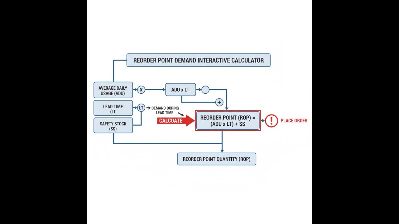
Visual Diagram

Reorder Point Demand Interactive Calculator
How to Use This Calculator
- Select your calculation mode from the dropdown — choose what you want to solve for (Reorder Point, Average Daily Demand, Lead Time, Safety Stock, Maximum Daily Demand, or Service Level Z-Score).
- Enter your Average Daily Demand in units per day and your Lead Time in days.
- Enter your Safety Stock in units — or, for the statistical method, enter your Demand Standard Deviation and Z-Score instead.
- Click Calculate to see your result.
Reorder Point Demand Interactive Visualizer
See how reorder point calculations balance lead time demand with safety stock to prevent stockouts. Adjust demand, lead time, and safety stock to visualize inventory levels and reorder timing.
REORDER POINT
550 units
LEAD TIME DEMAND
500 units
DAYS COVERAGE
5.5 days
FIRGELLI Automations — Interactive Engineering Calculators
Formulas & Equations
Use the formula below to calculate your reorder point.
Basic Reorder Point Formula
ROP = (D × L) + SS
ROP = Reorder Point (units)
D = Average Daily Demand (units/day)
L = Lead Time (days)
SS = Safety Stock (units)
Maximum Demand Method
ROP = (Dmax × Lmax)
SS = (Dmax × Lmax) - (Davg × Lavg)
Dmax = Maximum Daily Demand (units/day)
Lmax = Maximum Lead Time (days)
Davg = Average Daily Demand (units/day)
Lavg = Average Lead Time (days)
Service Level Method (Statistical)
SS = Z × σD × √L
ROP = (D × L) + (Z × σD × √L)
Z = Service Level Z-Score (dimensionless)
σD = Standard Deviation of Daily Demand (units/day)
√L = Square Root of Lead Time (days0.5)
Common Z-Scores:
Z = 1.28 → 90% service level
Z = 1.65 → 95% service level
Z = 2.33 → 99% service level
Days of Coverage
Days = ROP ÷ D
Days = Days of Inventory Coverage (days)
ROP = Reorder Point (units)
D = Average Daily Demand (units/day)
Simple Example
Average daily demand: 100 units/day. Lead time: 5 days. Safety stock: 50 units.
Lead time demand = 100 × 5 = 500 units. Reorder point = 500 + 50 = 550 units. Place a new order when stock drops to 550 units.
Theory & Engineering Applications
The reorder point represents the inventory threshold that triggers a replenishment order, balancing the competing objectives of maintaining service levels while minimizing working capital tied up in inventory. This fundamental inventory control parameter emerged from industrial engineering research in the mid-20th century and remains central to modern supply chain optimization, particularly in manufacturing environments where stockouts can halt entire production lines.
Fundamental Theory of Reorder Point Optimization
The basic reorder point formula ROP = (D × L) + SS consists of two distinct components serving different purposes. The lead time demand component (D × L) represents the expected consumption during the replenishment cycle—the inventory needed to sustain operations from the moment an order is placed until new stock arrives. The safety stock component (SS) provides a buffer against demand variability and supply uncertainty.
What many practitioners fail to recognize is that reorder point calculations inherently assume a continuous review system where inventory levels are monitored constantly. In periodic review systems where stock is checked at fixed intervals, the formula must be modified to account for the review period: ROP = D × (L + R) + SS, where R is the review period length. This distinction becomes critical in environments with weekly or monthly stock counts rather than perpetual inventory systems.
The safety stock component is not merely a buffer but a statistically derived quantity that directly determines service level performance. When using the service level method, the safety stock SS = Z × σD × √L incorporates demand variability through the standard deviation σD and acknowledges that uncertainty compounds over the lead time period through the square root relationship. The Z-score selection represents a fundamental business trade-off: higher service levels (larger Z values) exponentially increase holding costs while reducing stockout costs and lost sales.
Demand Variability and Lead Time Uncertainty
The statistical reorder point method assumes normally distributed demand, an assumption that frequently fails in real-world applications. Products with intermittent demand patterns, seasonal fluctuations, or promotional activities exhibit demand distributions with high kurtosis or skewness, rendering normal distribution-based safety stock calculations inadequate. Advanced practitioners employ bootstrap methods or empirical distribution analysis to capture actual demand patterns rather than relying on theoretical distributions.
Lead time variability compounds the complexity of reorder point determination. When both demand and lead time are variable, the safety stock formula becomes SS = Z × √(L × σD² + D² × σL²), where σL represents lead time standard deviation. This formulation, derived from variance propagation principles, reveals that lead time variability has a multiplicative effect proportional to average demand squared, making supplier reliability critically important for high-velocity items.
Manufacturing and Production Applications
In manufacturing environments, reorder points must account for batch sizing constraints and production scheduling realities. When supplier minimum order quantities exceed calculated reorder points, the effective ROP becomes the MOQ, potentially leading to saw-tooth inventory patterns with higher average inventory levels. Assembly operations with multiple components require coordinated reorder points across the bill of materials to prevent component shortages that can idle entire production lines.
The automotive industry pioneered kanban systems that implement reorder points through visual signals rather than numerical calculations. Each kanban card represents a fixed quantity, and the number of kanbans in circulation effectively sets the reorder point. This physical implementation makes inventory policies visible to shop floor workers and creates immediate feedback when consumption rates change, enabling rapid adjustments that purely computational systems may miss.
Multi-Echelon Inventory Considerations
In distribution networks with regional warehouses, distribution centers, and retail locations, reorder points at downstream locations affect optimal stocking levels at upstream facilities. A regional warehouse serving multiple retail stores must set its reorder point considering the aggregated demand patterns across all locations it serves, not merely the direct demand it experiences. The coefficient of variation (standard deviation divided by mean) generally decreases with demand aggregation, allowing lower relative safety stocks at centralized facilities—a phenomenon known as risk pooling.
The pharmaceutical industry demonstrates the critical importance of reorder point accuracy in regulated environments. Drug shortages can endanger patient safety, while excess inventory of temperature-sensitive medications leads to spoilage and waste. Pharmaceutical distributors often employ dual reorder points: a standard ROP for routine ordering and an emergency ROP that triggers expedited orders when inventory drops below critical levels, accepting higher transportation costs to prevent stockouts of essential medications.
Economic and Financial Implications
While reorder point calculations focus on operational parameters, the financial implications are substantial. The average inventory level in a reorder point system equals (Q/2) + SS, where Q is the order quantity. Since safety stock is held continuously, it represents permanent working capital investment that earns no return. A company with $100 million in inventory holding 30% as safety stock has tied up $30 million in buffer stock—capital that could fund expansion, research, or debt reduction.
The relationship between service level and safety stock is highly non-linear. Improving service level from 95% to 99% (Z-score from 1.65 to 2.33) increases safety stock by 41%, but the incremental stockout reduction is only 4 percentage points. This diminishing returns relationship means that pursuing very high service levels becomes exponentially expensive. Leading supply chain organizations segment their SKU portfolios, applying high service levels only to critical items while accepting lower service for slow-moving or easily substitutable products.
Worked Example: Electronic Component Distribution
Consider a distributor of microcontroller chips supplying electronics manufacturers. Historical data reveals the following parameters:
- Average daily demand: 847 units/day
- Standard deviation of daily demand: 126 units/day
- Average supplier lead time: 18 days
- Standard deviation of lead time: 3.2 days
- Target service level: 97.5% (Z = 1.96)
- Current inventory policy: Weekly review cycle
Step 1: Calculate Lead Time Demand
Lead time demand = D × L = 847 units/day × 18 days = 15,246 units
Step 2: Calculate Safety Stock with Demand and Lead Time Variability
Using the combined variability formula:
SS = Z × √(L × σD² + D² × σL²)
SS = 1.96 × √(18 × 126² + 847² × 3.2²)
SS = 1.96 × √(285,768 + 7,349,644)
SS = 1.96 × √7,635,412
SS = 1.96 × 2,763.4 = 5,416 units
Step 3: Account for Review Period
Since inventory is checked weekly (7 days), not continuously:
Effective lead time = L + R = 18 + 7 = 25 days
Revised lead time demand = 847 × 25 = 21,175 units
Revised safety stock with review period:
SS = 1.96 × √(25 × 126² + 847² × 3.2²)
SS = 1.96 × √(396,900 + 7,349,644)
SS = 1.96 × √7,746,544
SS = 1.96 × 2,783.3 = 5,455 units
Step 4: Calculate Reorder Point
ROP = Lead Time Demand + Safety Stock
ROP = 21,175 + 5,455 = 26,630 units
Step 5: Analyze Results
Days of coverage = 26,630 ÷ 847 = 31.4 days
Safety stock percentage = (5,455 ÷ 26,630) × 100 = 20.5%
This calculation reveals that the weekly review period adds 39 units to safety stock compared to continuous review (5,455 vs. 5,416), a 0.7% increase. However, the lead time variability component contributes 7,349,644 to the variance calculation while demand variability during lead time contributes only 396,900—demonstrating that supplier reliability has 18.5 times more impact than demand variability for this particular item. The distributor should prioritize supplier relationship management and possibly negotiate more consistent lead times rather than focusing solely on demand forecasting improvements.
If the distributor could reduce lead time standard deviation from 3.2 to 2.0 days while keeping all other parameters constant, safety stock would drop to 4,752 units—a reduction of 703 units or 12.9%. At a unit cost of $3.78 and an annual carrying cost rate of 24%, this improvement would free up $637 in annual carrying costs per SKU. Across 1,200 similar components, the total annual savings would exceed $764,000, justifying significant investment in supplier development programs.
For more specialized inventory calculations across various industries, explore our collection of engineering calculators covering production planning, material requirements, and supply chain optimization.
Practical Applications
Scenario: Medical Device Manufacturing
Jennifer manages procurement for a cardiac pacemaker manufacturer where a critical titanium housing component has a 14-day lead time from their Swiss supplier. Daily production consumes an average of 127 housings with a standard deviation of 18 units. Any stockout halts the entire assembly line and delays shipments of life-saving devices. Using the reorder point calculator with a 99% service level (Z = 2.33), she calculates ROP = (127 × 14) + (2.33 × 18 × √14) = 1,778 + 157 = 1,935 units. This means when inventory drops to 1,935 housings during the weekly count, purchasing immediately places a replenishment order. The 157-unit safety stock provides an 8.8% buffer above lead time demand, protecting against both demand spikes and occasional customs delays. This calculation directly supports the company's regulatory commitment to uninterrupted production of critical medical devices.
Scenario: Retail Chain Distribution Planning
Marcus oversees inventory for a regional grocery chain's distribution center supplying 47 stores with organic pasta. Average daily demand across the network is 2,340 packages with a supplier lead time of 6 days. However, the supplier occasionally experiences delays up to 9 days, and promotional activities can spike demand to 3,100 packages daily. Using the maximum demand method in the calculator, Marcus enters average demand of 2,340 units/day, average lead time of 6 days, maximum demand of 3,100 units/day, and maximum lead time of 9 days. The calculator determines safety stock of 13,860 units (the difference between worst-case usage of 27,900 and normal lead time demand of 14,040). This 99% buffer protects against the perfect storm of a supplier delay coinciding with a promotional surge, preventing out-of-stock situations that would disappoint health-conscious customers and damage the chain's fresh food reputation.
Scenario: Aerospace Fastener Supply
Robert manages specialized aerospace fasteners for aircraft assembly where a particular titanium bolt costs $47 each and usage averages 83 units per day with minimal variability. The domestic supplier maintains a 22-day lead time, and Robert's company targets 95% service level to balance inventory costs against line stoppage risk. He currently maintains a reorder point of 2,400 bolts but suspects it may be excessive. Using the calculator's "Calculate Safety Stock" mode, he enters average demand of 83 units/day, lead time of 22 days, and current ROP of 2,400 units. The calculator reveals his actual safety stock is 574 units—his ROP minus the 1,826 lead time demand. With the service level mode (Z = 1.65 for 95%), he discovers optimal safety stock should be approximately 300 units (using estimated demand standard deviation of 12 units/day). His current policy ties up an extra $12,878 in excess safety stock (274 units × $47), working capital that could be redeployed. By adjusting his reorder point to 2,126 units, he maintains the target service level while freeing significant cash for other operational needs.
Frequently Asked Questions
▶ What's the difference between reorder point and reorder quantity?
▶ How do I determine the right service level percentage for my products?
▶ Should I use average lead time or maximum lead time for reorder point calculations?
▶ How often should I recalculate reorder points?
▶ What should I do if my calculated reorder point is higher than my maximum inventory capacity?
▶ How do promotions and seasonal demand affect reorder point calculations?
Free Engineering Calculators
Explore our complete library of free engineering and physics calculators.
Browse All Calculators →🔗 Explore More Free Engineering Calculators
About the Author
Robbie Dickson — Chief Engineer & Founder, FIRGELLI Automations
Robbie Dickson brings over two decades of engineering expertise to FIRGELLI Automations. With a distinguished career at Rolls-Royce, BMW, and Ford, he has deep expertise in mechanical systems, actuator technology, and precision engineering.
Need to implement these calculations?
Explore the precision-engineered motion control solutions used by top engineers.


