Designing an optical system—whether a telescope, microscope, or machine vision camera—always comes down to one hard question: how fine a detail can you actually resolve? The answer is set by diffraction, not by your sensor or your glass quality. Use this Optical Resolution Rayleigh Calculator to calculate angular resolution, required aperture, linear resolution at distance, and more, using wavelength and aperture diameter as your primary inputs. Getting this right matters in astronomy, semiconductor inspection, surveillance imaging, and any application where resolving fine spatial detail is the whole point. This page includes the Rayleigh criterion formula, a worked satellite imaging example, theory behind the diffraction limit, and a full FAQ.
What is the Rayleigh criterion?
The Rayleigh criterion defines the minimum angular separation at which two point sources of light can be distinguished as separate by an optical system. It sets the fundamental resolution limit imposed by diffraction — the bending of light as it passes through an aperture.
Simple Explanation
Think of shining two small flashlights from far away. At some distance, they stop looking like 2 separate lights and blur into 1. The Rayleigh criterion tells you exactly where that boundary is — determined by the size of your lens and the wavelength (color) of the light. Bigger lens, shorter wavelength: sharper image. Smaller lens, longer wavelength: blurrier image. That's the whole idea.
📐 Browse all 1000+ Interactive Calculators
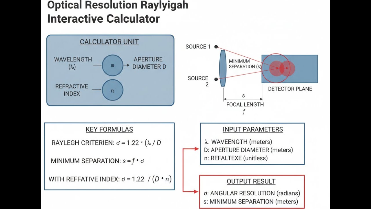
Optical Resolution Diagram

Interactive Rayleigh Resolution Calculator
How to Use This Calculator
- Select your calculation mode from the dropdown — angular resolution, required aperture, linear resolution, or one of the other options.
- Enter the wavelength of light in nanometers (e.g., 550 nm for green visible light).
- Enter the aperture diameter in millimeters, or the target resolution in arcseconds depending on your selected mode.
- Click Calculate to see your result.
Optical Resolution Rayleigh Interactive Visualizer
See how aperture size and wavelength determine the fundamental resolution limit of optical systems. Watch the Airy disk pattern and angular resolution change in real-time as you adjust parameters.
Angular Resolution
1.38"
Linear Resolution
6.7 mm
Resolving Power
149k
FIRGELLI Automations — Interactive Engineering Calculators
Rayleigh Criterion Equations
Use the formula below to calculate angular resolution using the Rayleigh criterion.
Angular Resolution (Rayleigh Criterion)
θ = 1.22 × λ / D
θ = angular resolution (radians)
λ = wavelength of light (meters)
D = aperture diameter (meters)
1.22 = constant derived from the first zero of the Bessel function J₁
Use the formula below to calculate linear resolution at a known distance.
Linear Resolution at Distance
d = θ × L
d = minimum resolvable linear separation (meters)
θ = angular resolution (radians)
L = distance to object (meters)
Use the formula below to calculate the minimum aperture diameter needed to hit a target resolution.
Required Aperture for Target Resolution
D = 1.22 × λ / θ
D = required aperture diameter (meters)
λ = wavelength of light (meters)
θ = desired angular resolution (radians)
Use the formula below to calculate the maximum distance at which two objects can be resolved.
Maximum Distance to Resolve Objects
Lmax = s / θ
Lmax = maximum distance (meters)
s = physical separation between objects (meters)
θ = angular resolution (radians)
Use the formula below to calculate resolving power for a given aperture and wavelength.
Resolving Power
R = D / (1.22 × λ)
R = resolving power (dimensionless)
D = aperture diameter (meters)
λ = wavelength of light (meters)
Simple Example
Wavelength: 550 nm (green light). Aperture diameter: 100 mm. Angular resolution: θ = 1.22 × 550×10⁻⁹ / 0.1 = 6.71×10⁻⁶ radians = 1.384 arcseconds. At a distance of 1000 m, the linear resolution is 6.71×10⁻⁶ × 1000 = 6.71 mm — the smallest feature you can distinguish at that range.
Theory & Engineering Applications
The Rayleigh criterion represents a fundamental limit on the resolution of any optical system imposed by the wave nature of light. When light passes through a circular aperture, diffraction creates an Airy disk pattern—a central bright disk surrounded by progressively dimmer rings. Lord Rayleigh proposed in 1879 that two point sources are just resolvable when the center of one Airy disk falls on the first minimum of the other. This produces a dip in intensity between the two peaks of approximately 26.3%, which human observers can reliably detect as two distinct sources rather than one blurred image.
Physical Origins of the Diffraction Limit
The factor 1.22 in the Rayleigh criterion arises from the mathematics of Fraunhofer diffraction through a circular aperture. The intensity distribution follows a Bessel function of the first kind, J₁(x), and the first zero occurs at x = 3.8317. When converted to angular terms for a circular aperture, this yields the coefficient 1.22 (specifically, 1.21966...). This is distinct from rectangular apertures, where the simple relation θ = λ/D applies without the 1.22 factor. Square or rectangular apertures produce different diffraction patterns with cross-shaped features rather than circular Airy rings.
Critically, the Rayleigh criterion assumes incoherent illumination—meaning the light from the two point sources has random phase relationships. For coherent sources (like two laser beams), interference patterns complicate the analysis and the simple Rayleigh criterion no longer applies. Additionally, the criterion assumes diffraction-limited performance: aberrations, atmospheric turbulence, manufacturing imperfections, or misalignment can degrade actual resolution far below the theoretical limit. A telescope's actual resolution is often limited by seeing conditions (atmospheric turbulence) rather than its diffraction limit, which is why adaptive optics systems have become essential for ground-based astronomy.
Wavelength Dependence and Multi-Spectral Systems
The linear dependence on wavelength means that resolution improves dramatically at shorter wavelengths. An optical microscope operating at λ = 400 nm (violet light) achieves 37% better resolution than the same instrument at λ = 700 nm (red light). This drives the use of ultraviolet microscopy, electron microscopy (effective wavelength ~0.0025 nm at 200 keV), and X-ray imaging for applications requiring extreme resolution. Conversely, radio telescopes operating at centimeter or meter wavelengths require enormous apertures to achieve modest angular resolution—hence the development of interferometric arrays like the Very Large Array (VLA) and the Event Horizon Telescope, which synthesize effective apertures spanning continents.
For multi-wavelength instruments, designers must balance competing requirements. A telescope optimized for visible light (550 nm) will underperform in the infrared (2000 nm) by a factor of 3.6 in angular resolution unless the aperture is correspondingly increased. Space telescopes like the James Webb Space Telescope employ a 6.5-meter primary mirror specifically to achieve high resolution at infrared wavelengths (0.6–28 μm), where its resolution still surpasses ground-based visible-light telescopes affected by atmospheric seeing.
Engineering Trade-offs in Optical Design
Aperture size directly controls resolution but introduces substantial engineering challenges. Larger apertures require heavier, more expensive optics with tighter manufacturing tolerances. The surface figure of a mirror must be accurate to approximately λ/20 (27.5 nm for visible light) to approach diffraction-limited performance. For a 10-meter telescope mirror, maintaining this tolerance across the entire surface represents an extraordinary manufacturing achievement. Weight scales with diameter cubed for constant aspect ratio, making large monolithic mirrors impractical beyond ~8 meters—hence the shift to segmented mirror designs like those in the Keck telescopes (36 hexagonal segments) and the James Webb Space Telescope (18 hexagonal segments).
Field of view (FOV) generally decreases as aperture increases for a given optical design. A large telescope with excellent resolution may only image a tiny patch of sky, necessitating either mosaic imaging (taking many exposures and stitching them together) or wide-field corrector optics that add complexity and cost. Camera lens designers face similar trade-offs: a 600mm f/4 telephoto lens provides excellent resolution but a narrow FOV, while a 24mm wide-angle lens covers a broad scene at the cost of lower angular resolution per pixel.
Microscopy and Near-Field Techniques
In microscopy, the Rayleigh criterion takes a modified form when using high-numerical-aperture objectives and oil immersion. The numerical aperture (NA) of a microscope objective is n·sin(α), where n is the refractive index of the medium between the objective and specimen, and α is the half-angle of the cone of light collected. The resolution becomes d = 0.61λ/NA for the Rayleigh criterion. With oil immersion (n ≈ 1.515) and high-angle objectives (NA up to 1.4), visible-light microscopes can resolve features down to approximately 200 nm—about half the wavelength of blue light.
Super-resolution techniques like STED microscopy, PALM, and STORM circumvent the diffraction limit through clever manipulation of fluorophore states, achieving resolutions down to 20 nm. These methods don't violate fundamental physics but instead exploit temporal or spectral separation to localize individual molecules with precision far exceeding classical resolution limits. Near-field scanning optical microscopy (NSOM) takes a different approach, positioning a sub-wavelength aperture within 10–20 nm of the sample surface, operating in the non-propagating evanescent field regime where the far-field diffraction limit doesn't apply.
Worked Example: Satellite Imaging Resolution
Consider a reconnaissance satellite in low Earth orbit designed to image ground targets. We need to determine the required aperture diameter to resolve objects 0.15 meters across from an orbital altitude of 425 km, using visible light at λ = 550 nm.
Step 1: Calculate required angular resolution
The angular size of the target is θtarget = d/L = 0.15 m / 425,000 m = 3.529 × 10⁻⁷ radians
Step 2: Apply Rayleigh criterion to find aperture
Rearranging θ = 1.22λ/D, we get D = 1.22λ/θ
D = 1.22 × (550 × 10⁻⁹ m) / (3.529 × 10⁻⁷ rad)
D = 6.71 × 10⁻⁷ m / 3.529 × 10⁻⁷ rad
D = 1.901 meters
Step 3: Verify resolution at operational distance
With D = 1.90 m and λ = 550 nm:
θ = 1.22 × (550 × 10⁻⁹) / 1.90 = 3.532 × 10⁻⁷ radians
Linear resolution at 425 km: d = θ × L = 3.532 × 10⁻⁷ × 425,000 m = 0.150 meters
Step 4: Convert angular resolution to practical units
θ in arcseconds = 3.532 × 10⁻⁷ rad × 206,265 arcsec/rad = 0.0729 arcseconds
Engineering reality check: A 1.9-meter aperture satellite telescope represents significant engineering complexity. The Hubble Space Telescope's 2.4-meter primary mirror provides context—our calculated satellite would need roughly 80% of Hubble's aperture diameter. Real reconnaissance satellites likely use even larger apertures (unconfirmed reports suggest 3–4 meters for modern systems) to overcome atmospheric turbulence effects and achieve better than Rayleigh-limited performance. Additionally, adaptive optics or deconvolution algorithms would be necessary to approach theoretical limits, as atmospheric turbulence, vibration, and thermal effects all degrade real-world performance.
The satellite would also need to consider motion blur during image acquisition: at 425 km altitude, orbital velocity is approximately 7.66 km/s, so exposure times must be kept extremely short (sub-millisecond) or image motion compensation employed to prevent blurring during capture.
Astronomical Applications and Interferometry
Radio astronomy demonstrates the extreme aperture requirements at long wavelengths. A single-dish radio telescope observing at λ = 21 cm (the hydrogen line) with a 100-meter diameter achieves angular resolution θ = 1.22 × 0.21 / 100 = 0.00256 radians = 8.85 arcminutes—roughly one-third the angular diameter of the Moon. This is completely inadequate for mapping galactic structure or studying distant objects. Radio interferometry solves this by combining signals from multiple telescopes separated by baselines up to thousands of kilometers, synthesizing an effective aperture equal to the maximum separation. The Very Long Baseline Array (VLBA) achieves baseline lengths of 8,600 km, providing milliarcsecond resolution at centimeter wavelengths—equivalent to reading newspaper headlines from across the country.
For further information on optical engineering principles, visit our comprehensive engineering calculator library, which includes tools for lens design, beam propagation, and photometric calculations.
Practical Applications
Scenario: Amateur Astronomer Selecting a Telescope
Marcus is an amateur astronomer deciding between a 6-inch (152 mm) and an 8-inch (203 mm) Schmidt-Cassegrain telescope for observing binary star systems. He wants to know if the additional cost of the larger aperture will allow him to resolve closer pairs. Using the Rayleigh calculator with λ = 550 nm (green light, to which human eyes are most sensitive), he finds the 6-inch scope provides 0.74 arcsecond resolution while the 8-inch achieves 0.55 arcseconds. Since many interesting binary systems have separations in the 0.6–1.0 arcsecond range, the 8-inch telescope will resolve approximately 35% more pairs under good seeing conditions. Marcus discovers that the theoretical improvement justifies the investment, though he also learns that local atmospheric seeing (typically 1–2 arcseconds at his suburban location) may limit practical performance, suggesting he should also consider observing sites with better conditions.
Scenario: Wildlife Photographer Planning Safari Equipment
Jennifer is a wildlife photographer preparing for a safari in Kenya and needs to determine if her 500mm f/4 lens (with a 125mm aperture diameter) can resolve sufficient feather detail on birds at typical shooting distances. She expects to photograph eagles and vultures at distances of 30–50 meters. Using the calculator with λ = 550 nm and D = 125 mm, she finds the angular resolution is 5.37 microradians (1.11 arcseconds). At 40 meters distance, this translates to a linear resolution of 0.215 mm—meaning she can theoretically resolve features like individual feather barbs. However, she also calculates that a 600mm f/4 lens (150mm aperture) would improve resolution to 0.179 mm at the same distance, a 17% improvement. This analysis helps her decide whether the significant weight and cost increase of the 600mm lens justifies the modest resolution gain, or whether cropping her 500mm images would be more practical for her needs.
Scenario: Optical Engineer Designing Inspection System
Dr. Patel is designing a machine vision system to inspect semiconductor wafer defects at a production facility. The system must resolve defects as small as 2.5 micrometers at a working distance of 150mm using blue LED illumination (λ = 470 nm) to maximize resolution. Using the Rayleigh calculator in "required aperture" mode, he calculates that the angular resolution needed is 2.5 μm / 150 mm = 16.67 microradians (3.44 arcseconds). This requires a minimum aperture diameter of 34.4 mm. Dr. Patel specifies a 40mm diameter lens system with a numerical aperture of 0.13 to provide some safety margin above the theoretical minimum. He also recognizes that the Rayleigh criterion represents an ideal case, so he plans for additional testing with practical considerations like vibration isolation, precise focus control (depth of field at this resolution is only ±12 micrometers), and proper illumination geometry to achieve maximum contrast on defects. The calculator has given him the fundamental limit, allowing him to set realistic performance targets and justify the budget for precision optics.
Frequently Asked Questions
Free Engineering Calculators
Explore our complete library of free engineering and physics calculators.
Browse All Calculators →🔗 Explore More Free Engineering Calculators
About the Author
Robbie Dickson — Chief Engineer & Founder, FIRGELLI Automations
Robbie Dickson brings over two decades of engineering expertise to FIRGELLI Automations. With a distinguished career at Rolls-Royce, BMW, and Ford, he has deep expertise in mechanical systems, actuator technology, and precision engineering.
Need to implement these calculations?
Explore the precision-engineered motion control solutions used by top engineers.


