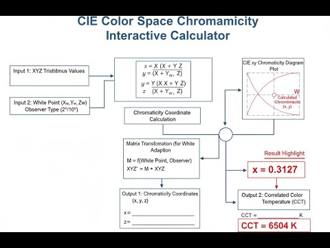
Specifying color accurately across manufacturing, display calibration, and lighting design means working in a common mathematical framework — and that framework is the CIE color space. Without it, a "warm white" LED from one supplier looks nothing like the same spec from another. Use this CIE Color Space Chromaticity Calculator to calculate chromaticity coordinates, tristimulus values, sRGB conversions, and correlated color temperature using XYZ values, RGB inputs, or dominant wavelength. It matters in LED manufacturing, display engineering, and colorimetry research — anywhere color consistency is a hard requirement, not a preference. This page includes the core formulas, a worked LED binning example, theory, and FAQ.
What is CIE Chromaticity?
CIE chromaticity is a way to describe the color of a light source using 2 numbers — x and y — that capture hue and saturation independently of how bright the light is. It's the international standard for communicating color across industries, from LED production to monitor calibration.
Simple Explanation
Think of chromaticity like describing the shade of paint on a wall, separate from how bright the room is. You can say a paint is "warm orange" without knowing if the light is dim or blazing — that's what chromaticity does for light. The CIE system turns that description into precise numbers so engineers, manufacturers, and scientists all mean exactly the same thing when they specify a color.
📐 Browse all 1000+ Interactive Calculators
Table of Contents
CIE Chromaticity Diagram

Interactive Calculator
How to Use This Calculator
- Select your calculation mode from the dropdown — choose from XYZ to chromaticity, RGB conversions, dominant wavelength, or CCT.
- Enter the required input values for your chosen mode (XYZ tristimulus values, RGB values 0–255, wavelength in nm, or xy chromaticity coordinates).
- Use the "Try Example" button to load a pre-filled set of values if you want to see a sample result first.
- Click Calculate to see your result.
CIE Color Space Chromaticity Interactive Visualizer
Visualize how XYZ tristimulus values map to chromaticity coordinates on the CIE 1931 diagram. Watch how changing input values moves your point through the horseshoe-shaped color gamut and see real-time RGB conversions.
x CHROMATICITY
0.410
y CHROMATICITY
0.360
CCT (K)
2856
FIRGELLI Automations — Interactive Engineering Calculators
Equations & Formulas
Use the formula below to calculate chromaticity coordinates from XYZ tristimulus values.
XYZ to Chromaticity Coordinates
x = X / (X + Y + Z)
y = Y / (X + Y + Z)
z = Z / (X + Y + Z) = 1 − x − y
Where X, Y, Z are CIE tristimulus values (dimensionless), and x, y, z are chromaticity coordinates (dimensionless, sum to unity).
Use the formula below to calculate tristimulus values from chromaticity coordinates and luminance.
Chromaticity to Tristimulus Values
X = (x / y) × Y
Z = [(1 − x − y) / y] × Y
Given chromaticity coordinates (x, y) and luminance Y, reconstruct full tristimulus values. Note: y ≠ 0 required.
Use the formula below to calculate sRGB values from XYZ tristimulus values.
XYZ to sRGB Transformation (D65)
Rlinear = 3.2405X − 1.5371Y − 0.4985Z
Glinear = −0.9693X + 1.8760Y + 0.0416Z
Blinear = 0.0556X − 0.2040Y + 1.0572Z
RsRGB = γ(Rlinear) × 255
Where γ(u) = 12.92u for u ≤ 0.0031308, else 1.055u1/2.4 − 0.055. Values clipped to [0, 255].
Use the formula below to calculate XYZ tristimulus values from sRGB inputs.
sRGB to XYZ Transformation
Rlinear = γ−1(RsRGB / 255)
X = 0.4124Rlinear + 0.3576Glinear + 0.1804Blinear
Y = 0.2127Rlinear + 0.7152Glinear + 0.0722Blinear
Z = 0.0193Rlinear + 0.1192Glinear + 0.9503Blinear
Where γ−1(u) = u/12.92 for u ≤ 0.04045, else [(u + 0.055)/1.055]2.4.
Use the formula below to calculate correlated color temperature from chromaticity coordinates.
McCamy's CCT Approximation
n = (x − 0.3320) / (0.1858 − y)
CCT = 449n³ + 3525n² + 6823.3n + 5520.33
Where CCT is correlated color temperature in Kelvin. Valid for approximately 2000 K to 10000 K near Planckian locus.
Simple Example
Given: X = 0.5, Y = 0.4, Z = 0.1 (XYZ to chromaticity mode)
Sum = 0.5 + 0.4 + 0.1 = 1.0
x = 0.5 / 1.0 = 0.500000
y = 0.4 / 1.0 = 0.400000
z = 0.1 / 1.0 = 0.100000
Theory & Engineering Applications
The CIE (Commission Internationale de l'Éclairage) color spaces represent the most fundamental framework for quantifying human color perception. Developed from the 1931 standard observer color matching experiments, the CIE XYZ tristimulus system mathematically describes any visible color as a weighted combination of three primary stimuli. The chromaticity diagram reduces this three-dimensional color space to a two-dimensional representation by normalizing out luminance, creating the horseshoe-shaped gamut familiar to every color scientist.
Tristimulus Values and the Fundamental Observer
The XYZ tristimulus values derive from the spectral power distribution of a light source convolved with the CIE 1931 standard observer color matching functions x̄(λ), ȳ(λ), and z̄(λ). For a spectral radiance L(λ), the tristimulus values are calculated as:
X = k ∫ L(λ) x̄(λ) dλ
where the integral spans the visible spectrum (typically 380-780 nm) and k is a normalization constant. The Y tristimulus value is specifically constructed to represent photometric luminance, making it directly proportional to perceived brightness. This dual role—serving both as a component of color specification and as an absolute measure of brightness—makes Y unique among the tristimulus values.
A critical but often overlooked limitation: the CIE 1931 standard observer represents the average color matching behavior of only 17 observers, all with normal color vision and 2° field of view. Real-world color perception varies significantly with field size (the CIE 1964 10° observer addresses this), observer age (lens yellowing shifts blue perception), and individual variation in cone photopigment sensitivity. High-precision colorimetry in applications like medical imaging or art reproduction must account for these observer metamerism effects.
Chromaticity Coordinates: Projection to the xy Plane
The transformation from tristimulus values to chromaticity coordinates represents a projective mapping that eliminates luminance information while preserving hue and saturation relationships. The normalization x + y + z = 1 means only two coordinates are independent; conventionally, x and y are reported while z is implicitly 1 − x − y. This projection collapses the three-dimensional color solid onto a two-dimensional plane, creating the iconic chromaticity diagram.
The spectral locus—the curved boundary of the diagram—represents monochromatic (single-wavelength) light sources from approximately 380 nm (violet) through 780 nm (deep red). The straight line connecting the spectral endpoints is the "line of purples," representing non-spectral colors formed by mixing extreme violet and red wavelengths. All physically realizable colors lie within or on this boundary; points outside represent imaginary colors with negative tristimulus values, mathematically valid but physically impossible to produce.
The white point location depends on the illuminant. D65 (x = 0.3127, y = 0.3290) represents average daylight at 6500 K and serves as the reference white for sRGB and most display technologies. Illuminant A (x = 0.4476, y = 0.4074) represents tungsten incandescent lighting at 2856 K. The shift in white point dramatically affects color rendering; a photograph taken under tungsten light appears orange when viewed under daylight without white balance correction.
Color Gamut and the RGB Transformation
The sRGB color space, standardized in IEC 61966-2-1, defines a specific triangular gamut within the CIE xy chromaticity diagram. The primaries are located at Red (0.6400, 0.3300), Green (0.3000, 0.6000), and Blue (0.1500, 0.0600), with D65 as the white point. The 3×3 transformation matrix connecting XYZ to linear RGB derives from solving the system of equations that maps these primaries and white point between coordinate systems.
The gamma correction applied in sRGB is not a simple power law. The piecewise function with a linear segment near zero (u ≤ 0.0031308) prevents infinite slope at the origin, which would amplify quantization noise in dark regions. The gamma exponent of 2.4 in the power law region approximates the inverse of typical CRT display response (gamma ≈ 2.2), though modern displays use lookup tables for precise calibration. This nonlinear encoding efficiently allocates the limited number of digital code values (256 per channel in 8-bit RGB) according to the Weber-Fechner law of human brightness perception.
Colors outside the sRGB gamut cannot be accurately reproduced on standard monitors. When converting from XYZ to RGB, negative linear RGB values or values exceeding 1.0 indicate out-of-gamut colors. The calculator clips these to [0, 1] before quantization, but this destroys color relationships.
Professional color management systems use gamut mapping algorithms—perceptual, relative colorimetric, absolute colorimetric, or saturation rendering intents—to preserve image appearance when mapping between gamuts. Simple clipping, while computationally trivial, produces the worst perceptual results.
Correlated Color Temperature and the Planckian Locus
The Planckian locus traces the chromaticity coordinates of blackbody radiators at temperatures from approximately 1000 K (deep red) to infinity (approaching D65 and beyond toward bluish-white). Correlated color temperature (CCT) describes how "warm" or "cool" a light appears by finding the temperature of the Planckian radiator whose chromaticity lies closest to the measured chromaticity. McCamy's formula provides a computationally efficient approximation valid near the Planckian locus, though iterative methods using Robertson's or Hernández-Andrés' algorithms achieve higher accuracy for research-grade colorimetry.
An often-misunderstood subtlety: CCT only has physical meaning for chromaticities near the Planckian locus. For deeply saturated colors (highly chromatic light sources), CCT becomes essentially meaningless—there is no "correlated color temperature" of a saturated red LED. The concept applies primarily to white and near-white illuminants. Additionally, equal CCT does not guarantee identical color rendering; two light sources at 3000 K can have vastly different spectral power distributions, leading to different Color Rendering Index (CRI) values and metameric effects on colored objects.
Industrial Application: Display Calibration and Color Management
Modern display manufacturing relies on chromaticity measurements at multiple points in the production pipeline. After LED backlight assembly, spectroradiometers measure the white point chromaticity and luminance uniformity across the panel. Deviations from the target D65 white point exceeding Δu'v' = 0.005 in the CIE 1976 UCS diagram (a perceptually uniform transformation of the xy diagram) are typically rejected for professional monitors. The transformation to u'v' coordinates weights chromaticity differences according to human discrimination thresholds—equal distances in u'v' space correspond to approximately equal perceived color differences, unlike the highly non-uniform xy space.
Color management systems in operating systems and applications use ICC profiles containing transformation matrices and lookup tables to map between device RGB spaces and the profile connection space (PCS), typically CIE XYZ or CIE L*a*b*. When an image moves from a wide-gamut camera (ProPhoto RGB) to a standard monitor (sRGB) to a printer (CMYK with device-specific gamut), each transformation must preserve perceptual appearance while handling out-of-gamut colors gracefully. The complexity of this color pipeline—often involving five or more color space transformations—demands rigorous chromaticity calculation at each step.
Worked Example: LED Color Binning
An LED manufacturer produces white LEDs for architectural lighting targeted at CCT = 3000 K ± 150 K (warm white). Quality control measures a production sample with the following tristimulus values: X = 0.3847, Y = 0.3512, Z = 0.1763. Determine if this LED meets specification.
Step 1: Calculate chromaticity coordinates from tristimulus values.
Sum = X + Y + Z = 0.3847 + 0.3512 + 0.1763 = 0.9122
x = X / Sum = 0.3847 / 0.9122 = 0.4217
y = Y / Sum = 0.3512 / 0.9122 = 0.3850
Step 2: Calculate CCT using McCamy's approximation.
n = (x − 0.3320) / (0.1858 − y) = (0.4217 − 0.3320) / (0.1858 − 0.3850)
n = 0.0897 / (−0.1992) = −0.4502
CCT = 449n³ + 3525n² + 6823.3n + 5520.33
CCT = 449(−0.4502)³ + 3525(−0.4502)² + 6823.3(−0.4502) + 5520.33
CCT = 449(−0.0913) + 3525(0.2027) + 6823.3(−0.4502) + 5520.33
CCT = −41.0 + 714.5 − 3071.9 + 5520.33 = 3121.9 K
Step 3: Compare to specification.
Target: 3000 K ± 150 K → acceptable range [2850 K, 3150 K]
Measured: 3121.9 K ✓ PASS
Step 4: Calculate distance from Planckian locus (Duv) for complete characterization.
For precise work, transform to u'v' coordinates: u' = 4X/(X + 15Y + 3Z), v' = 9Y/(X + 15Y + 3Z)
u' = 4(0.3847) / (0.3847 + 15(0.3512) + 3(0.1763)) = 1.5388 / 6.1817 = 0.2490
v' = 9(0.3512) / 6.1817 = 3.1608 / 6.1817 = 0.5115
The Planckian locus at 3122 K has u'BB ≈ 0.2523, v'BB ≈ 0.5193
Duv = [(u' − u'BB)² + (v' − v'BB)²]0.5
Duv = [(0.2490 − 0.2523)² + (0.5115 − 0.5193)²]0.5
Duv = [(−0.0033)² + (−0.0078)²]0.5 = [1.089×10⁻⁵ + 6.084×10⁻⁵]0.5 = 0.0084
The LED meets the CCT specification. The Duv value of 0.0084 indicates the chromaticity lies slightly below the Planckian locus (negative Duv, appearing slightly greenish), which is typical for phosphor-converted white LEDs. ANSI C78.377 specifies quadrangles around target CCT points with Duv tolerances; for precise binning, this LED's (CCT, Duv) coordinates would be plotted against the acceptance quadrangle boundaries.
This calculation demonstrates why manufacturers cannot rely solely on CCT for LED binning. Two LEDs at identical CCT but different Duv values appear visibly different in hue—one greenish, one pinkish. Multi-dimensional binning using both CCT and Duv coordinates ensures color consistency in lighting installations.
For more color and optical engineering calculations, visit our comprehensive engineering calculator library.
Practical Applications
Scenario: Display Manufacturing Quality Control
Jessica, a display engineer at an OLED panel manufacturing facility, needs to verify that the white point of a production batch meets the sRGB specification for computer monitors. Using a spectroradiometer, she measures the tristimulus values of the panel's D65 white at maximum brightness: X = 89.47, Y = 94.38, Z = 102.81. She uses the CIE chromaticity calculator to convert these values to xy coordinates, obtaining x = 0.3119, y = 0.3289. Comparing against the D65 target of (0.3127, 0.3290), she calculates the chromaticity error: Δx = 0.0008, Δy = 0.0001, well within the ±0.003 tolerance for professional displays. The batch passes QC and proceeds to final assembly, ensuring customers receive accurately calibrated monitors for color-critical work.
Scenario: Architectural Lighting Design
Marco, a lighting designer for a museum renovation, must specify LED fixtures that provide warm white illumination at 2700 K while maintaining high color rendering for artwork. The manufacturer provides specification sheets listing chromaticity coordinates (x = 0.4578, y = 0.4101) for their museum-grade LEDs. Marco uses the chromaticity to CCT calculator, which returns 2687 K—close to the target. However, he also calculates the distance from the Planckian locus in u'v' space and finds Duv = +0.0023, indicating a slightly pinkish tint above the blackbody curve. This positive Duv is acceptable for museum applications where slight warmth enhances the appearance of paintings and textiles. He specifies this LED bin for the 300+ fixtures in the gallery spaces, ensuring consistent, flattering illumination throughout the museum.
Scenario: Spectroscopy and Color Science Research
Dr. Aisha, a vision scientist studying color perception under narrow-band LED illumination, measures the spectral power distribution of a 530 nm green LED using her spectrometer. The software outputs CIE XYZ values of (0.1847, 0.6782, 0.1194) after integrating the measured spectrum with the 1931 standard observer color matching functions. To visualize where this stimulus falls on the chromaticity diagram relative to the spectral locus, she converts to xy coordinates using the calculator: x = 0.1891, y = 0.6946. Plotting this point, she confirms it lies very close to the spectral locus near 530 nm, as expected for a narrow-band LED. She then uses the dominant wavelength calculation mode to verify that observers would perceive this as 529.3 nm monochromatic light, validating her LED source for psychophysical experiments on wavelength discrimination thresholds.
Frequently Asked Questions
Free Engineering Calculators
Explore our complete library of free engineering and physics calculators.
Browse All Calculators →🔗 Explore More Free Engineering Calculators
About the Author
Robbie Dickson — Chief Engineer & Founder, FIRGELLI Automations
Robbie Dickson brings over two decades of engineering expertise to FIRGELLI Automations. With a distinguished career at Rolls-Royce, BMW, and Ford, he has deep expertise in mechanical systems, actuator technology, and precision engineering.
Need to implement these calculations?
Explore the precision-engineered motion control solutions used by top engineers.


