Positioning a lens correctly — whether for a camera, microscope, or machine vision system — requires knowing exactly how object distance, image distance, and focal length interact. Use this Thin Lens Equation Interactive Calculator to calculate image distance, object distance, focal length, magnification, or lens power using any two known optical parameters. Getting these relationships right matters in cameras, telescopes, eyeglasses, robotic guidance systems, and industrial inspection rigs. This page covers the governing formula, a worked engineering example, optical theory, and a full FAQ.
What is the thin lens equation?
The thin lens equation is a formula that links how far an object is from a lens, how far the resulting image forms on the other side, and the lens's focal length. Know any 2 of those 3 values and you can solve for the third.
Simple Explanation
Think of a magnifying glass held over a piece of paper on a sunny day — move it up and down until the light spot is sharpest. That sweet spot is the focal point. The thin lens equation is just the math that tells you exactly where that sharp image forms based on where the object is and the strength of the lens. Closer object, farther image — and the formula keeps track of all of it.
📐 Browse all 1000+ Interactive Calculators
How to Use This Calculator
- Select your calculation mode from the dropdown — choose which parameter you want to solve for (image distance, object distance, focal length, magnification, lens power, or complete analysis).
- Enter the known values into the visible input fields — object distance, image distance, focal length, and/or object height depending on your selected mode, all in millimeters.
- If you want to test the calculator quickly, click Try Example to pre-fill realistic values for the current mode.
- Click Calculate to see your result.
Ray Diagram

Interactive Calculator
Thin Lens Equation Interactive Visualizer
Visualize how object distance, image distance, and focal length interact in real-time using the thin lens equation. Watch the light rays bend through the lens and see exactly where your image forms as you adjust optical parameters.
IMAGE DISTANCE
200 mm
MAGNIFICATION
-1.0×
LENS POWER
10.0 D
FIRGELLI Automations — Interactive Engineering Calculators
Governing Equations
Use the formula below to calculate image distance, object distance, or focal length from any 2 known values.
Thin Lens Equation (Gaussian Form)
1/f = 1/do + 1/di
f = focal length (mm) — distance from lens to focal point
do = object distance (mm) — distance from object to lens
di = image distance (mm) — distance from lens to image
Use the formula below to calculate lateral magnification and image height.
Magnification Equations
M = -di/do = hi/ho
M = lateral magnification (dimensionless)
ho = object height (mm)
hi = image height (mm)
Negative magnification indicates inverted image
Use the formula below to calculate lens power in diopters from focal length.
Lens Power (Diopters)
P = 1/f
P = lens power (diopters, D)
f = focal length (meters)
Positive power = converging lens, Negative power = diverging lens
Use the formula below to calculate image position using distances measured from the focal points rather than the lens center.
Newtonian Form (Alternative)
xo · xi = f2
xo = distance from object to front focal point (mm)
xi = distance from back focal point to image (mm)
Useful when measuring from focal points rather than lens center
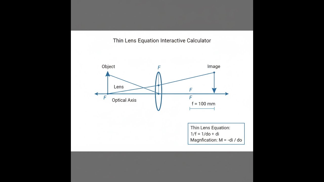
Simple Example
Object distance (do): 200 mm
Focal length (f): 100 mm
Solving for image distance: 1/di = 1/100 − 1/200 = 0.005, so di = 200 mm
Magnification: M = −200/200 = −1.0x (real, inverted, same size as object)
Theory & Practical Applications
Geometric Optics Foundation
The thin lens equation represents one of the most fundamental relationships in geometric optics, governing image formation for lenses where the thickness is negligible compared to the radii of curvature. This paraxial approximation assumes rays make small angles with the optical axis—typically less than 10 degrees—and permits linear mathematical treatment of ray trajectories. Real optical systems deviate from this ideal behavior through spherical aberration, coma, astigmatism, field curvature, and distortion, collectively known as Seidel aberrations. For precision applications like semiconductor lithography or high-resolution microscopy, engineers must account for these aberrations through multi-element designs and aspherical surfaces.
The sign conventions are critical for correct application. In the standard Cartesian convention, distances measured in the direction of light propagation are positive. For a converging (convex) lens with positive focal length, a real object (do positive) produces a real inverted image (di positive) when the object distance exceeds the focal length. When the object lies inside the focal point (do less than f), the image becomes virtual (di negative), upright, and enlarged—the principle behind magnifying glasses. Diverging (concave) lenses with negative focal length always produce virtual, upright, reduced images for real objects. This behavior makes diverging lenses essential for correcting myopia in eyeglasses and for expanding laser beams in beam delivery systems.
Critical Distance Relationships
The relationship between object and image distances exhibits several operationally significant boundaries. When the object resides at exactly twice the focal length (do = 2f), the image forms at the same distance on the opposite side (di = 2f) with unity magnification but inverted. This symmetric configuration minimizes certain optical aberrations and finds application in relay optics and telecentric imaging systems. As the object approaches the focal point, the image distance increases toward infinity—the working principle of collimators that produce parallel light beams. At the focal point itself (do = f), the lens equation predicts infinite image distance, meaning rays emerge parallel.
Machine vision engineers exploit the hyperbolic nature of the thin lens relationship when designing optical inspection systems. For a 25mm focal length lens imaging a circuit board at 100mm working distance, the image forms at 33.33mm behind the lens with -0.333x magnification. Reducing the working distance to 75mm shifts the image plane to 37.5mm with -0.5x magnification. This 4.17mm sensor displacement requires precise mechanical focus adjustment or depth-of-field management through aperture control. Industrial systems often employ motorized focus stages with sub-micron positioning to maintain critical focus across varying part geometries.
Power and Diopters in Optical Design
Lens power expressed in diopters (reciprocal meters) provides an additive quantity for thin lens combinations. A +5D spectacle lens combined with a +3D reading lens yields +8D total power, assuming negligible separation. This additivity simplifies optometric prescriptions and optical system design. However, thick lens combinations or separated elements require the more complex principal plane formulation where effective focal length depends on element spacing. Telephoto camera lenses exploit this principle by combining positive and negative groups to achieve long focal lengths in compact mechanical packages.
The practical limit of the thin lens approximation appears when lens thickness reaches approximately 10% of the diameter or 5% of the focal length. Beyond these thresholds, principal plane locations shift significantly from the geometric center. A 50mm diameter, 10mm thick biconvex lens with 100mm focal length exhibits principal plane separation of roughly 3.3mm, introducing measurable errors in image distance predictions if treated as infinitely thin. Precision optical designers use matrix methods (ABCD matrices or ray transfer matrices) to accurately model thick lens systems and multi-element assemblies.
Real-World Engineering Applications
Smartphone camera modules demonstrate sophisticated thin lens engineering within extreme space constraints. A typical wide-angle phone camera employs a 4.5mm focal length lens array positioned 5.8mm from the 1/2.55" sensor (5.57mm diagonal). For infinity focus (do approaching infinity), the thin lens equation yields di ≈ f = 4.5mm. However, the mechanical sensor-to-lens distance must account for the lens group thickness and back focal distance. To focus on a subject 250mm away (typical arm's length for selfies), the image distance increases to 4.582mm, requiring only 82 microns of focus travel. Voice coil motor actuators provide this precise adjustment in under 100 milliseconds for fast autofocus performance.
Laser materials processing systems utilize carefully designed focusing optics to achieve the power densities necessary for cutting, welding, and marking. A 1070nm fiber laser with 10mm beam diameter requires focusing to approximately 50 micron spot size for precision micromachining. Using a 163mm focal length lens, the thin lens equation combined with Gaussian beam optics predicts the focused spot diameter and Rayleigh range. The depth of focus—the axial range over which the beam remains below twice the minimum spot area—determines the maximum workpiece thickness variation the system tolerates. Engineers selecting focusing optics must balance focal length against working distance, numerical aperture, and chromatic aberration to optimize processing results across different materials and thicknesses.
Projection systems in data projectors and home theater equipment rely on precision lens design to magnify small microdisplay panels (typically 0.55" to 0.7" diagonal) to screen images exceeding 100 inches. A projector with 1.5:1 throw ratio positioned 150 inches from a screen produces a 100-inch diagonal image. The required focal length and lens-to-panel distance follow from the thin lens equation with appropriate scaling for the actual sensor dimensions. Modern projectors incorporate zoom lenses (variable focal length) and lens shift mechanisms to accommodate different installation geometries without image keystoning. The design must also manage chromatic aberration—wavelength-dependent focal length variation—which would otherwise produce colored fringing in high-contrast regions.
Worked Example: Industrial Machine Vision System Design
An automotive component inspection system requires imaging 18mm diameter bearing races at 3.2 micron/pixel resolution for surface defect detection. The production line mandates 300mm working distance to provide clearance for part handling mechanisms and lighting. Calculate the required focal length, sensor format, magnification, and depth of field for f/5.6 aperture.
Step 1: Determine Required Magnification
Sensor pixel size: 3.2 μm
Field of view required: 18mm diameter (use 20mm with margin)
Sensor width needed: horizontal pixel count = 20mm / 0.0032mm = 6250 pixels
Select 2/3" format sensor: 8.8mm × 6.6mm, 2752 × 2064 pixels (3.2μm pixels)
Actual magnification: M = sensor width / field width = 8.8mm / 20mm = 0.44x
Step 2: Calculate Image Distance
From magnification: M = -di / do
0.44 = -di / 300mm
di = -132mm (negative indicates real image on opposite side)
Using absolute value: di = 132mm
Step 3: Calculate Focal Length
1/f = 1/do + 1/di
1/f = 1/300 + 1/132
1/f = 0.003333 + 0.007576 = 0.010909
f = 91.67mm
Select standard focal length: 90mm (closest available)
Step 4: Verify Actual Performance with Standard Lens
With f = 90mm, do = 300mm:
1/di = 1/f - 1/do = 1/90 - 1/300 = 0.01111 - 0.00333 = 0.00778
di = 128.6mm
Actual magnification: M = -128.6/300 = -0.429x
Actual field of view: 8.8mm / 0.429 = 20.5mm (acceptable)
Step 5: Calculate Depth of Field
For f/5.6 aperture, circle of confusion c = 2 × pixel size = 6.4μm
DOF = 2 × c × N × (do/M)2 / f2
DOF = 2 × 0.0064 × 5.6 × (300/0.429)2 / 902
DOF = 0.0717 × 488,400 / 8100 = 4.32mm
This 4.32mm depth of field provides adequate tolerance for bearing race thickness variation (typically ±1.5mm) while maintaining critical 3.2μm resolution. The inspection system can reliably detect surface defects as small as 10μm across the full part surface. For improved depth of field at cost of reduced light throughput, stopping down to f/8 would increase DOF to 8.7mm, though this requires brighter illumination or longer exposure times that may limit inspection speed.
Edge Cases and Failure Modes
The thin lens equation breaks down under several conditions that practicing engineers must recognize. When object distance equals focal length (do = f), the equation predicts infinite image distance—rays emerge parallel, forming no focused image. This condition appears during collimator alignment and focus adjustment in afocal systems. Attempting to solve for image distance numerically near this singularity produces numerical instability unless proper limiting behavior is implemented. Similarly, for diverging lenses with real objects, the virtual image forms on the same side as the object (negative di), which can confuse sign conventions if not carefully tracked.
Chromatic aberration—wavelength-dependent focal length variation—fundamentally limits achromatic lens performance. Crown glass with Abbe number 58 exhibits roughly 1% focal length difference between blue (486nm) and red (656nm) wavelengths. For a 100mm focal length lens, this 1mm focal shift causes color fringing in images. Achromatic doublets combining crown and flint glass elements reduce this error to approximately 0.1mm, while apochromatic triplets achieve 0.01mm correction across wider spectral ranges. Broadband applications from UV through near-IR require sophisticated multi-element designs or reflective optics that exhibit no chromatic aberration. You can explore more optical and mechanical design principles in our comprehensive free engineering calculator library.
Frequently Asked Questions
▼ Why does my calculated image distance become negative?
▼ How do I account for lens thickness in precision applications?
▼ What happens when the object is exactly at the focal point?
▼ How does aperture (f-number) affect image formation calculations?
▼ Can I use the thin lens equation for compound lens systems?
▼ Why do camera lenses use focal length instead of diopters?
Free Engineering Calculators
Explore our complete library of free engineering and physics calculators.
Browse All Calculators →🔗 Explore More Free Engineering Calculators
About the Author
Robbie Dickson — Chief Engineer & Founder, FIRGELLI Automations
Robbie Dickson brings over two decades of engineering expertise to FIRGELLI Automations. With a distinguished career at Rolls-Royce, BMW, and Ford, he has deep expertise in mechanical systems, actuator technology, and precision engineering.
Need to implement these calculations?
Explore the precision-engineered motion control solutions used by top engineers.


