Sizing a piping system without accounting for friction losses is how you end up with undersized pumps, starved flow rates, and expensive redesigns after installation. Use this Darcy-Weisbach calculator to calculate head loss, pipe diameter, flow velocity, friction factor, volumetric flow rate, or required pipe length using friction factor, pipe geometry, and fluid properties. It matters across HVAC design, municipal water distribution, chemical process engineering, and oil and gas pipelines. This page includes the governing equations, a worked municipal water design example, flow regime theory, and a full FAQ.
What is the Darcy-Weisbach equation?
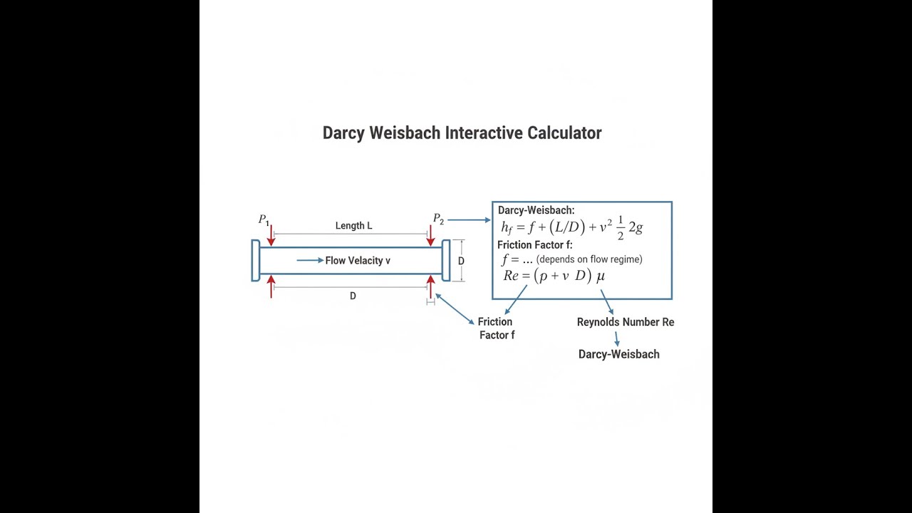
The Darcy-Weisbach equation calculates how much pressure or head is lost due to friction when a fluid flows through a pipe. Give it the pipe length, diameter, flow velocity, and friction factor — it tells you the energy your pump needs to overcome.
Simple Explanation
Think of it like pushing water through a garden hose: the longer the hose, the narrower it is, and the faster the water moves, the harder you have to push. The Darcy-Weisbach equation puts an exact number on that resistance — the "friction head loss" — so you can size your pump or pipe correctly before anything gets built.
📐 Browse all 1000+ Interactive Calculators
System Diagram

Interactive Calculator
How to Use This Calculator
- Select your Calculation Mode from the dropdown — choose what you want to solve for (head loss, diameter, velocity, friction factor, flow rate, or pipe length).
- Enter the known values into the visible input fields: friction factor, pipe length, pipe diameter, flow velocity, kinematic viscosity, and pipe roughness as applicable.
- If your mode requires head loss or flow rate as an input, enter those values in the corresponding fields.
- Click Calculate to see your result.
Darcy-Weisbach interactive visualizer
Visualize how friction factor, pipe geometry, and flow velocity affect head loss in real-time. Adjust parameters to see immediate changes in pressure drop, flow regime, and energy requirements.
HEAD LOSS
5.10 m
REYNOLDS
200,000
PRESSURE
50 kPa
FIRGELLI Automations — Interactive Engineering Calculators
Governing Equations
Use the formula below to calculate head loss due to friction in a pipe.
Darcy-Weisbach Equation
hf = f · (L / D) · (v² / 2g)
Where:
- hf = head loss due to friction (m)
- f = Darcy friction factor (dimensionless)
- L = pipe length (m)
- D = pipe diameter (m)
- v = mean flow velocity (m/s)
- g = gravitational acceleration (9.81 m/s²)
Reynolds Number
Re = (v · D) / ν
Where:
- Re = Reynolds number (dimensionless)
- ν = kinematic viscosity (m²/s)
Flow regimes: Laminar (Re < 2300), Transitional (2300 ≤ Re ≤ 4000), Turbulent (Re > 4000)
Pressure Drop
ΔP = ρ · g · hf
Where:
- ΔP = pressure drop (Pa)
- ρ = fluid density (kg/m³, typically 1000 kg/m³ for water)
Volumetric Flow Rate
Q = v · A = v · (π · D² / 4)
Where:
- Q = volumetric flow rate (m³/s)
- A = pipe cross-sectional area (m²)
Relative Roughness
ε/D = ε / D
Where:
- ε = absolute pipe roughness (m)
- ε/D = relative roughness (dimensionless)
Simple Example
Given: f = 0.02, L = 100 m, D = 100 mm (0.1 m), v = 2 m/s, g = 9.81 m/s²
Formula: hf = f · (L/D) · (v²/2g)
Calculation: hf = 0.02 × (100/0.1) × (4/19.62)
Result: hf = 0.02 × 1000 × 0.204 = 4.08 m
Theory & Practical Applications
The Darcy-Weisbach equation represents one of the most fundamental relationships in fluid mechanics, quantifying the irreversible energy loss that occurs when a viscous fluid flows through a pipe. Unlike the empirical Hazen-Williams equation which is restricted to water at specific temperature ranges, the Darcy-Weisbach formulation applies universally to any Newtonian fluid in any circular conduit, making it the preferred choice for rigorous engineering analysis across petroleum, chemical processing, HVAC, and municipal water systems.
Fundamental Physics and Flow Regimes
At its core, the Darcy-Weisbach equation captures the conversion of mechanical energy (pressure head) into thermal energy through viscous dissipation at the pipe wall and turbulent momentum exchange within the flow field. The friction factor f encodes the complex physics of boundary layer development, turbulent eddies, and surface roughness interaction. For laminar flow (Re < 2300), the friction factor follows the analytical Poiseuille solution: f = 64/Re, completely independent of surface roughness because viscous forces dominate and fluid particles maintain orderly parallel streamlines that never contact the wall asperities.
The critical insight most engineers overlook is that the transition region (2300 ≤ Re ≤ 4000) is not merely a smooth interpolation between laminar and turbulent correlations — it represents a fundamentally unstable flow condition where small disturbances can trigger intermittent bursts of turbulence. Operating industrial systems in this regime should be avoided when possible because the friction factor becomes unpredictable and sensitive to vibration, valve operation upstream, and even changes in ambient temperature affecting fluid viscosity.
In practice, municipal water distribution networks naturally operate well into the turbulent regime (Re typically 10⁵ to 10⁶), while viscous oils in chemical plants may deliberately maintain laminar flow to minimize mixing and preserve stratification.
The Moody Diagram and Implicit Friction Factor Determination
For turbulent flow, determining the friction factor requires solving the implicit Colebrook-White equation, which relates f to both Reynolds number and relative roughness ε/D. The iterative nature of this calculation historically necessitated the Moody diagram — a graphical solution that practicing engineers memorized and relied upon for decades. Modern computational tools eliminate this manual lookup, but understanding the Moody diagram's structure reveals critical design insights. Notice that at very high Reynolds numbers (Re > 10⁶), the friction factor curves become horizontal, meaning f depends only on relative roughness — the flow becomes "fully rough" and viscous effects negligible. This explains why increasing pump speed to raise Re in an already-turbulent rough pipe yields diminishing returns in head loss reduction.
The practical implication surfaces immediately in pipe material selection. For a 150 mm diameter water main, commercial steel (ε ≈ 0.045 mm) gives ε/D = 0.0003, while PVC (ε ≈ 0.0015 mm) yields ε/D = 0.00001 — a 30-fold difference. At Re = 500,000, this translates to f = 0.0185 for steel versus f = 0.0138 for PVC, meaning the steel pipe requires 34% more pumping power for identical flow rate. Over a 20-year system lifetime, this energy penalty far exceeds the material cost differential, which is why modern municipal specifications increasingly mandate plastic piping for non-potable applications.
Scale Effects and the Economic Pipe Diameter Problem
The Darcy-Weisbach equation exposes a non-intuitive scaling relationship: head loss varies as v²/D, but flow rate Q scales as v·D². If we double the pipe diameter while maintaining constant flow rate, velocity drops by a factor of four (since A quadruples), and head loss decreases by a factor of 32 (velocity squared effect times diameter increase). This cubic-law scaling creates the fundamental engineering trade-off: larger pipes dramatically reduce friction losses but incur higher capital costs for material, excavation, and support structures. The optimal economic diameter balances present-value pumping energy costs against amortized installation expenses, typically yielding velocities in the range of 1.5-3.0 m/s for water distribution networks.
For long-distance pipelines, this optimization becomes critical. The Trans-Alaska Pipeline System (TAPS) transports crude oil 1,300 km through 1,220 mm diameter pipe at approximately 2.5 m/s. The friction factor for this flow (Re ≈ 250,000) is approximately 0.015, producing a head loss of roughly 750 m over the pipeline length. This requires twelve pump stations positioned along the route, each providing approximately 60 m of head. Had the designers selected 915 mm pipe (the next smaller standard size), head loss would have increased by a factor of six (diameter reduction cubed, velocity increase squared), necessitating proportionally more pumping infrastructure and consuming an additional 150 MW of continuous power — equivalent to a medium-sized power plant operating 24/7 solely to overcome friction.
Industrial Applications Across Engineering Domains
In HVAC system design, duct friction calculations using the Darcy-Weisbach equation determine the pressure rise requirement for air handling units. Commercial buildings typically target air velocities of 6-10 m/s in supply ducts to balance acoustic concerns (higher velocities generate noise) against duct size (lower velocities require larger cross-sections that consume valuable ceiling plenum space). For a 40,000 m² office building with a 300 m equivalent duct length and 8 m/s velocity in 400 mm ducts, the friction factor (Re ≈ 210,000, smooth duct) is approximately 0.016, yielding a head loss of 245 Pa. This represents nearly 40% of the total fan static pressure in a properly designed system, with the remainder consumed by filters, coils, dampers, and terminal units.
Chemical process engineers encounter the Darcy-Weisbach equation in reactor feed systems where precise flow control is mandatory. A 50 m pipe run delivering a proprietary catalyst slurry at 12 L/s through a 75 mm schedule 40 stainless steel pipe (ID = 77.9 mm) at 60°C experiences unique challenges. The slurry's apparent kinematic viscosity of 8.5×10⁻⁶ m²/s produces Re = 110,000 — solidly turbulent but low enough that the transition to laminar flow could occur if temperature drops even slightly, altering viscosity.
With stainless steel roughness ε = 0.045 mm (relative roughness 0.00058), the friction factor is 0.022, producing 1.87 m of head loss. More critically, if a heat exchanger failure reduces fluid temperature to 40°C, viscosity doubles, Reynolds number halves to 55,000, friction factor increases to 0.028, and head loss jumps to 2.38 m — a 27% increase that could starve the downstream reactor and trigger a process upset. This sensitivity explains why process industries install flow meters with closed-loop control rather than relying on fixed-speed pumps and passive resistance.
Worked Example: Municipal Water Distribution System Design
Consider designing a water supply line for a new residential development requiring 315 L/s peak flow delivered through a 2.4 km ductile iron main (ε = 0.26 mm). The municipal engineer must select between 400 mm, 450 mm, or 500 mm nominal diameter pipe, each with different material cost, installation complexity, and long-term energy consumption.
Step 1: Calculate flow velocities for each diameter option
For 400 mm pipe (D = 0.400 m):
A = π(0.400)²/4 = 0.1257 m²
v = Q/A = 0.315/0.1257 = 2.506 m/s
For 450 mm pipe (D = 0.450 m):
A = π(0.450)²/4 = 0.1590 m²
v = 0.315/0.1590 = 1.981 m/s
For 500 mm pipe (D = 0.500 m):
A = π(0.500)²/4 = 0.1963 m²
v = 0.315/0.1963 = 1.604 m/s
Step 2: Determine Reynolds numbers and flow regimes
Using kinematic viscosity ν = 1.0×10⁻⁶ m²/s for water at 20°C:
For 400 mm: Re = (2.506 × 0.400) / 1.0×10⁻⁶ = 1,002,400 (turbulent)
For 450 mm: Re = (1.981 × 0.450) / 1.0×10⁻⁶ = 891,450 (turbulent)
For 500 mm: Re = (1.604 × 0.500) / 1.0×10⁻⁶ = 802,000 (turbulent)
Step 3: Calculate relative roughness and friction factors
For 400 mm: ε/D = 0.00026/0.400 = 0.00065
Using Colebrook-White (or Moody diagram): f ≈ 0.0192
For 450 mm: ε/D = 0.00026/0.450 = 0.00058
f ≈ 0.0188
For 500 mm: ε/D = 0.00026/0.500 = 0.00052
f ≈ 0.0185
Step 4: Apply Darcy-Weisbach equation to calculate head losses
For 400 mm pipe:
hf = 0.0192 × (2400/0.400) × (2.506²)/(2×9.81) = 0.0192 × 6000 × 0.3203 = 36.89 m
For 450 mm pipe:
hf = 0.0188 × (2400/0.450) × (1.981²)/(2×9.81) = 0.0188 × 5333 × 0.2002 = 20.07 m
For 500 mm pipe:
hf = 0.0185 × (2400/0.500) × (1.604²)/(2×9.81) = 0.0185 × 4800 × 0.1312 = 11.65 m
Step 5: Calculate pressure drops and pumping power requirements
ΔP = ρghf, with ρ = 1000 kg/m³:
For 400 mm: ΔP = 1000 × 9.81 × 36.89 = 361.9 kPa
Power = ΔP × Q / η = 361,900 × 0.315 / 0.75 = 152.0 kW
For 450 mm: ΔP = 1000 × 9.81 × 20.07 = 196.9 kPa
Power = 196,900 × 0.315 / 0.75 = 82.7 kW
For 500 mm: ΔP = 1000 × 9.81 × 11.65 = 114.3 kPa
Power = 114,300 × 0.315 / 0.75 = 48.0 kW
Step 6: Economic analysis and selection
Assuming electricity costs $0.12/kWh and 6000 hours annual operation at peak flow (25% duty cycle with peaking factor):
400 mm annual energy cost: 152.0 kW × 6000 hrs × $0.12 = $109,440
450 mm annual energy cost: 82.7 kW × 6000 hrs × $0.12 = $59,544
500 mm annual energy cost: 48.0 kW × 6000 hrs × $0.12 = $34,560
The 20-year present value difference between 400 mm and 500 mm options is approximately $950,000 in energy costs alone (assuming 3% discount rate). Even if the 500 mm pipe costs $400,000 more to purchase and install than the 400 mm option, the lifecycle cost analysis strongly favors the larger diameter. This example demonstrates why proper application of the Darcy-Weisbach equation directly impacts multi-million dollar infrastructure decisions.
This analysis assumes constant friction factor, but in reality, ductile iron pipes experience progressive roughness increase as corrosion products accumulate. After 20 years in aggressive water chemistry, effective roughness may triple to ε = 0.78 mm, increasing friction factors to 0.0265 (400 mm) and 0.0215 (500 mm), with corresponding head loss increases of 38% and 16% respectively. The larger pipe's lower relative roughness makes it more resilient to aging effects, providing additional long-term value beyond the initial calculation suggests.
Advanced Considerations and Limitations
The standard Darcy-Weisbach formulation assumes fully developed, steady flow in straight pipes with circular cross-sections. Real piping systems contain valves, fittings, bends, reducers, and branches — each contributing localized head losses that must be added to the friction losses. These minor losses are typically expressed as equivalent lengths (Leq = K·D/f, where K is the loss coefficient) or added directly as velocity head multiples. For complex systems with numerous fittings, minor losses can exceed pipe friction losses, making accurate K-factor selection critical.
Non-Newtonian fluids require modified friction factor correlations. Power-law fluids (like polymer solutions) exhibit viscosity dependent on shear rate, necessitating the Dodge-Metzner correlation. Slurries with high solids content experience additional head loss from particle-particle and particle-wall interactions not captured by the clean-fluid Darcy-Weisbach equation. These applications require empirical adjustments or computational fluid dynamics analysis for accurate design.
For more engineering resources including pipe sizing tools, pump selection calculators, and hydraulic system analyzers, visit the FIRGELLI Engineering Calculator Library.
Frequently Asked Questions
Free Engineering Calculators
Explore our complete library of free engineering and physics calculators.
Browse All Calculators →🔗 Explore More Free Engineering Calculators
- Pipe Flow Velocity Calculator
- Reynolds Number Calculator — Laminar or Turbulent
- Hydraulic Pump Flow Rate Calculator
- Cylinder Volume Calculator — Tank Pipe Capacity
- Cv Flow Calculator
- Darcys Law Calculator
- Mean Free Path Calculator
- Friction Force Calculator — Static and Kinetic
- Water Hammer Pressure Calculator
- Projectile Motion Calculator
About the Author
Robbie Dickson — Chief Engineer & Founder, FIRGELLI Automations
Robbie Dickson brings over two decades of engineering expertise to FIRGELLI Automations. With a distinguished career at Rolls-Royce, BMW, and Ford, he has deep expertise in mechanical systems, actuator technology, and precision engineering.
Need to implement these calculations?
Explore the precision-engineered motion control solutions used by top engineers.


