Coefficient Of Discharge Interactive Calculator

The Coefficient of Discharge (Cd) is a dimensionless parameter that quantifies the flow efficiency of orifices, nozzles, venturi meters, weirs, and other flow-measuring devices. It represents the ratio of actual discharge to theoretical discharge, accounting for energy losses due to viscosity, turbulence, vena contracta formation, and boundary layer effects. Engineers in hydraulic system design, water resource management, chemical processing, and aerospace propulsion rely on accurate Cd values to predict flow rates, calibrate instruments, and optimize fluid delivery systems.

📐 Browse all free engineering calculators

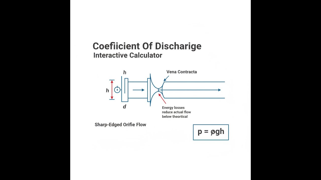
Flow Through Orifice Diagram

Interactive Calculator

Governing Equations

Theory & Practical Applications

Physical Mechanisms Governing Discharge Coefficient

The coefficient of discharge quantifies the cumulative effect of three distinct physical phenomena that reduce actual flow below the idealized prediction from Bernoulli's equation. First, the vena contracta effect causes the fluid jet to contract downstream of the orifice opening as streamlines converge toward the centerline. At the vena contracta location (typically 0.5-1.0 orifice diameters downstream for sharp-edged orifices), the jet cross-sectional area reaches approximately 62-64% of the orifice area, a phenomenon captured by the coefficient of contraction (C_c). Second, viscous boundary layer losses near the orifice walls dissipate kinetic energy, reducing the average velocity across the jet cross-section. This is quantified by the coefficient of velocity (C_v), which compares actual average velocity to theoretical velocity. The discharge coefficient is the product: C_d = C_c × C_v. For sharp-edged orifices in turbulent flow (Re greater than 10,000), typical values are C_c ≈ 0.64 and C_v ≈ 0.97, yielding C_d ≈ 0.62.

A critical non-obvious factor is the Reynolds number dependence of the discharge coefficient. While turbulent flow produces relatively stable C_d values, transitional and laminar regimes (Re below 10,000) exhibit significant C_d variation. For sharp-edged orifices at Re = 1,000, C_d can drop to 0.58-0.59 due to enhanced viscous dissipation and altered separation patterns. This poses calibration challenges in microfluidic devices, precision dosing systems for pharmaceuticals, and low-velocity hydraulic testing where operating conditions span both laminar and turbulent regimes. Engineers must either maintain turbulent flow through geometric design or apply Reynolds-corrected C_d correlations such as the Lichtarowicz equation: C_d = C_d,∞ + K/Re^0.5, where C_d,∞ is the fully turbulent asymptote and K is an empirically determined constant.

Orifice Geometry and Discharge Coefficient Variations

The discharge coefficient is highly sensitive to orifice edge geometry. Sharp-edged orifices (thickness less than 0.1d with 90-degree entry angle) produce C_d ≈ 0.60-0.62 due to maximum flow separation and vena contracta contraction. Rounded entrance orifices with radius r/d = 0.1-0.2 suppress separation, reducing vena contracta effects and increasing C_d to 0.85-0.95. Chamfered orifices (45-degree entrance bevel) yield intermediate values of C_d ≈ 0.72-0.78. Re-entrant or Borda mouthpieces, where the orifice tube extends inward into the reservoir, actually decrease C_d to approximately 0.52 due to recirculation zones inside the tube that further contract the effective flow area.

For thick-plate orifices where wall thickness exceeds two diameters, the flow pattern transitions from a free jet to pipe flow. Once the jet reattaches to the tube walls (L/d greater than 2.5), the discharge coefficient approaches unity (C_d ≈ 0.96-0.99) because the orifice behaves as a short tube rather than an orifice plate. This distinction is critical in fuel injector design, hydraulic valve sizing, and spray nozzle applications where a few millimeters of additional length can alter flow rate by 30-40% at constant pressure drop.

Industrial Applications Across Sectors

In water distribution and wastewater treatment, discharge coefficients govern the calibration of flow measurement devices including orifice plates (C_d ≈ 0.60-0.61 per ISO 5167), venturi meters (C_d ≈ 0.95-0.98), and flow nozzles (C_d ≈ 0.96-0.99). Municipal water utilities rely on orifice plate flow meters to monitor discharge from reservoirs and pumping stations, with accuracy requirements of ±2% necessitating precise C_d determination through in-situ calibration against weigh tank or ultrasonic reference standards. Wastewater overflow weirs use C_d values ranging from 0.58-0.65 depending on edge sharpness and approach velocity, with systematic underprediction of flow during storm events when debris accumulation rounds the weir edge and artificially inflates C_d.

In aerospace propulsion, fuel injector orifices in gas turbine combustors operate under extreme conditions where C_d directly controls fuel-air ratio and combustion efficiency. Jet engine fuel nozzles incorporate arrays of 30-100 micro-orifices (diameter 0.3-0.8 mm) operating at pressure drops of 50-150 bar. Manufacturers measure C_d for each nozzle under simulated operating conditions (heated Jet-A fuel at 150°C, cavitation number σ less than 1.5) to ensure flow uniformity within ±3% across the array. Cavitation inception inside these orifices can increase apparent C_d by 10-15% due to vapor core formation that reduces effective flow area, requiring cavitation-resistant designs with rounded entrances or flow conditioners.

In chemical process industries, orifice restrictors control dosing rates for reactants, catalysts, and pH adjustment chemicals. Pharmaceutical batch reactors use calibrated orifice flow controllers with C_d stability better than ±1% over six months to maintain product consistency. A subtle issue arises with non-Newtonian fluids (polymer solutions, slurries, emulsions) where apparent viscosity varies with shear rate. The discharge coefficient becomes concentration-dependent and non-constant across the operating range, necessitating empirical correlation development: C_d = f(Re, Ca), where Ca is the cavitation number accounting for vapor pressure effects at high velocities.

Worked Example: Hydraulic System Design

Problem: A mobile hydraulic excavator uses an orifice-based flow divider to split pump output between the boom cylinder (priority circuit) and auxiliary functions. The pump delivers 180 L/min at 210 bar operating pressure. The flow divider employs a sharp-edged orifice to bypass 45 L/min to the auxiliary circuit when boom demand is below maximum. Design the orifice diameter assuming water-glycol hydraulic fluid (ρ = 1065 kg/m³, μ = 0.048 Pa·s at 50°C operating temperature) and verify that the Reynolds number supports the assumed discharge coefficient of 0.61.

Solution:

Step 1: Convert flow rate to SI units
Q_actual = 45 L/min = 45 × 10^-3 / 60 = 7.50 × 10^-4 m³/s

Step 2: Determine pressure drop across orifice
The orifice drops from system pressure (210 bar) to tank return pressure (assumed 5 bar):
Δp = 210 - 5 = 205 bar = 2.05 × 10⁷ Pa

Step 3: Calculate hydraulic head equivalent
Using Bernoulli: Δp = ρgh, so h = Δp / (ρg) = 2.05 × 10⁷ / (1065 × 9.81) = 1962 m equivalent head

Step 4: Determine theoretical velocity
V_theoretical = √(2gh) = √(2 × 9.81 × 1962) = 196.2 m/s

Step 5: Calculate actual velocity
V_actual = C_d × V_theoretical = 0.61 × 196.2 = 119.7 m/s

Step 6: Solve for orifice area
Q_actual = A × V_actual, so A = Q_actual / V_actual = 7.50 × 10^-4 / 119.7 = 6.27 × 10^-6 m²

Step 7: Calculate orifice diameter
A = πd²/4, so d = √(4A/π) = √(4 × 6.27 × 10^-6 / π) = 2.82 × 10^-3 m = 2.82 mm

Step 8: Verify Reynolds number assumption
Re = ρVd/μ = (1065 × 119.7 × 2.82 × 10^-3) / 0.048 = 7.49 × 10⁶

Verification: Reynolds number of 7.49 million confirms fully turbulent flow, well above the Re greater than 10⁴ threshold for stable C_d = 0.61 in sharp-edged orifices. The design is valid.

Step 9: Design margin analysis
Actual flow with standard 3.0 mm drill bit: A = π(0.003)²/4 = 7.07 × 10^-6 m²
Q = C_d × A × √(2gh) = 0.61 × 7.07 × 10^-6 × 196.2 = 8.46 × 10^-4 m³/s = 50.8 L/min

The standard 3.0 mm orifice delivers 13% more flow than the target 45 L/min. To hit specification, either select the calculated 2.82 mm size (requiring precision reaming) or use a 3.0 mm orifice with upstream pressure regulation to reduce Δp from 205 bar to 161 bar: Q ∝ √Δp, so (45/50.8)² × 205 = 161 bar required differential.

Advanced Considerations and Limitations

Discharge coefficients exhibit temperature sensitivity through viscosity dependence. Hydraulic oils decrease in viscosity by 50-70% from cold start (0°C) to operating temperature (60°C), shifting Reynolds number by a factor of 2-3. Systems designed with C_d calibrated at operating temperature may experience 5-8% flow increase during warm-up if operating in the transitional regime (Re = 5,000-20,000). Critical applications require temperature-compensated flow control or viscosity-independent devices like turbine meters.

The phenomenon of discharge coefficient hysteresis occurs when orifice edges experience erosion, corrosion, or deposition. Abrasive slurries can round sharp edges over months of operation, gradually increasing C_d from 0.60 to 0.75-0.80, causing systematic flow overprediction. Conversely, scale deposition in hard water systems reduces effective diameter, decreasing flow capacity by 10-30% while nominally maintaining C_d relative to the reduced area. Periodic inspection and recalibration are essential for custody transfer applications where financial implications demand ±0.5% accuracy.

For compressible flow applications (gases, steam, multiphase fluids), the discharge coefficient becomes a function of pressure ratio β = p₂/p₁. When β falls below 0.85, the standard incompressible C_d values require correction factors derived from ISO 5167 or AGA Report No. 3. Choked flow conditions (β below critical pressure ratio of approximately 0.53 for air) impose maximum flow limits regardless of downstream pressure, a regime where discharge coefficient concepts must be replaced by critical flow function analysis. More information on engineering flow calculations can be found at the FIRGELLI engineering calculator hub.

Frequently Asked Questions