Inverse Square Law Interactive Calculator

The inverse square law describes how physical quantities like light intensity, sound pressure, gravitational force, and electromagnetic radiation diminish with distance from a point source. This fundamental relationship—intensity decreasing proportionally to the square of the distance—governs everything from photographic lighting setups to radiation safety protocols in medical imaging. Engineers, photographers, acousticians, and radiation safety officers rely on precise inverse square calculations to predict field strengths, optimize sensor placement, and ensure compliance with exposure limits.

📐 Browse all free engineering calculators

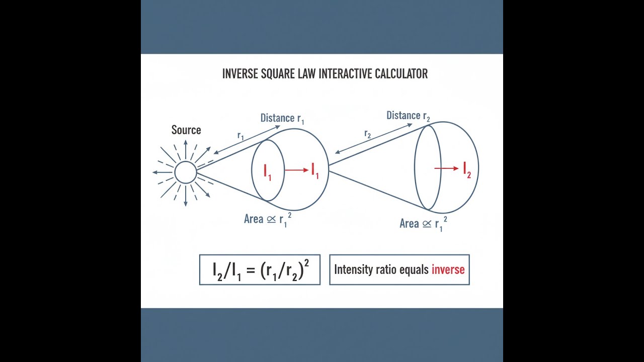
Inverse Square Law Diagram

Interactive Inverse Square Law Calculator

Governing Equations

Theory & Practical Applications

Physical Foundation of the Inverse Square Law

The inverse square law emerges directly from geometric dilution of energy or field strength spreading spherically from a point source. When a source radiates uniformly in all directions, the total emitted power P must pass through every spherical surface centered on the source, regardless of radius. Since the surface area of a sphere scales as 4πr², and the same total power spreads over progressively larger areas at greater distances, the intensity (power per unit area) necessarily decreases as 1/r². This relationship is not an empirical observation but a mathematical consequence of three-dimensional Euclidean geometry combined with energy conservation.

The law applies rigorously only to ideal point sources in free space with no absorption or scattering. Real sources have finite extent, which introduces near-field deviations where the source cannot be approximated as a point. The transition from near-field to far-field behavior occurs at distances exceeding several times the largest source dimension. Additionally, atmospheric absorption, humidity, and particulate scattering cause faster-than-inverse-square intensity decay for electromagnetic and acoustic radiation propagating through real media. Professional measurements account for these non-ideal effects through correction factors derived from transmission coefficients specific to wavelength and propagation medium.

Applications in Photographic and Cinematographic Lighting

Professional photographers and cinematographers exploit the inverse square law to control illumination gradients and depth-of-field rendering. A portrait lit by a close softbox exhibits rapid light falloff across the subject's face—moving from nose to ears might traverse 0.15 m, which at a 0.6 m source distance represents a 25% distance increase and therefore a 36% intensity reduction (ratio of 0.64). This dramatic gradient creates dimensionality and separation from background. Conversely, a distant key light at 4 m produces nearly uniform illumination across the same facial span, as the 0.15 m depth represents only 3.75% distance variation and less than 8% intensity change.

In commercial product photography, lighting ratios between key and fill sources are precisely calculated using inverse square predictions. A three-light setup might specify key at 1 m providing I_key, fill at 2 m providing I_key/4, and rim at 0.7 m providing approximately 2× I_key. The photographer adjusts these distances rather than power settings to maintain color temperature consistency while achieving specific contrast ratios. This technique is particularly critical in automotive and jewelry photography where specular highlights must be controlled within sensor dynamic range limitations of 12-14 stops for high-end digital backs.

Radiation Safety and Medical Dosimetry

In diagnostic radiology and radiation therapy, the inverse square law governs both patient dose optimization and operator protection. Fluoroscopy procedures require real-time X-ray imaging, exposing interventional radiologists to scattered radiation. Moving from 0.5 m to 1.0 m from the scatter source reduces exposure to 25% of the original rate—a critical safety margin during multi-hour procedures. The ALARA principle (As Low As Reasonably Achievable) incorporates inverse square calculations into procedural planning, specifying minimum operator distances for various beam intensities and exposure durations.

Brachytherapy source placement demonstrates precise dosimetric applications. An iridium-192 seed delivering 10 Gy/hr at 1 cm produces only 2.5 Gy/hr at 2 cm and 1.11 Gy/hr at 3 cm. Treatment planning systems calculate isodose curves accounting for tissue heterogeneity, but the fundamental inverse square geometry determines the steep dose gradient that enables tumor targeting while sparing adjacent healthy tissue. Seeds must be positioned with sub-millimeter accuracy because 1 mm displacement at 5 mm nominal distance represents 20% distance error and 36% dose error—potentially the difference between tumor control and treatment failure.

Acoustic Engineering and Sound Reinforcement

Sound pressure levels follow inverse square behavior in the direct field of loudspeakers before reverberant field dominates in enclosed spaces. Outdoor concert sound systems must account for inverse square attenuation when specifying array configurations for even coverage. A line array approximates a line source in the near field (intensity decreasing as 1/r rather than 1/r²), transitioning to point source behavior beyond the array length. This extended near-field region—where intensity decreases only 3 dB per doubling distance instead of 6 dB—enables even SPL distribution across audience areas spanning 50-100 m depth.

In architectural acoustics, the critical distance r_c marks where direct and reverberant sound pressures are equal. Beyond r_c, the inverse square law no longer predicts SPL decay because diffuse reflections dominate. For a source with directivity factor Q in a room with reverberation time T60 and volume V, r_c = 0.057 × √(QV/T60). A typical conference room might have r_c = 1.8 m, meaning inverse square predictions hold only within this radius—critical for microphone placement in recording and teleconferencing applications.

Electromagnetic Compliance Testing and Antenna Analysis

RF electromagnetic interference (EMI) measurements at regulatory test facilities employ inverse square corrections when comparing near-field probe data to far-field compliance limits. A circuit radiating unintentional emissions measured at 3 m distance must meet limits specified at 10 m for Class B equipment. If the 3 m measurement yields 45 dBμV/m, the predicted 10 m level is 45 - 20log₁₀(10/3) = 34.5 dBμV/m, assuming far-field conditions apply. This extrapolation is valid only when measurement distance exceeds 2D²/λ where D is the largest radiating dimension and λ is wavelength—ensuring spherical wave propagation rather than near-field reactive components.

Antenna gain measurements utilize inverse square relationships to calibrate absolute power density. A reference antenna with known gain G_ref produces power density S = (P_t × G_ref)/(4πr²) at distance r, where P_t is transmitter power. Measuring received signal strength from an unknown antenna at the same position and input power allows gain determination by comparison. Professional antenna ranges maintain far-field distances exceeding 2D²/λ, which for a 2 m aperture at 10 GHz requires r ≥ 267 m—necessitating elevated or compact range configurations with collimating reflectors.

Worked Example: Multi-Stage Lighting Design

Problem: A theater lighting designer must illuminate a 2.4 m wide backdrop to achieve 500 lux at center while maintaining maximum 15% intensity variation across the width. The existing inventory includes 2000 W tungsten-halogen Fresnels with 85% lamp-to-beam efficiency. Determine the required fixture distance, verify uniformity, calculate power density at the fixture position, and assess whether moving the fixture 0.5 m closer would maintain acceptable uniformity while achieving higher center intensity.

Given:

• Target center illuminance: I_center = 500 lux
• Backdrop width: w = 2.4 m
• Maximum intensity variation: ±15% (intensity ratio 0.85 to 1.0 at edges relative to center)
• Fixture power: P_total = 2000 W × 0.85 = 1700 W effective
• Assume isotropic radiation for initial calculation (will verify with cosine falloff)

Solution Part 1: Determine fixture distance for center illuminance

Using I = P/(4πr²), solve for r:

r = √[P/(4π×I_center)] = √[1700 W/(4π × 500 W/m²)]

r = √[1700/(6283.2)] = √0.2706 = 0.520 m

This distance would apply for perpendicular incidence at center. For a flat backdrop, we must account for oblique angles at edges.

Solution Part 2: Verify edge uniformity with geometric correction

At the backdrop edge 1.2 m from center, the distance from fixture to edge point is:

r_edge = √(r² + 1.2²) = √(0.520² + 1.44) = √1.710 = 1.308 m

Intensity at edge (inverse square only): I_edge = I_center × (r/r_edge)² = 500 × (0.520/1.308)² = 500 × 0.158 = 79.0 lux

This represents 15.8% of center intensity—far below the 85% requirement. The issue is that placing the fixture at 0.52 m creates severe geometric non-uniformity. We need to increase fixture distance substantially.

For acceptable edge uniformity, require I_edge/I_center ≥ 0.85. Using combined inverse square and cosine law (intensity ∝ cos θ/r² for Lambertian source):

At edge: cos θ_edge = r/r_edge, so I_edge = I_center × (r/r_edge)³ for perpendicular illumination geometry

Setting I_edge/I_center = 0.85:

0.85 = (r/√(r² + 1.44))³

Let x = r²: 0.85 = (x/(x + 1.44))^1.5

0.85^(2/3) = x/(x + 1.44)

0.8987 = x/(x + 1.44)

0.8987x + 1.294 = x

x = 12.78, therefore r = 3.57 m

Solution Part 3: Calculate actual center intensity at 3.57 m

I_center = 1700/(4π × 3.57²) = 1700/159.9 = 10.6 lux

This is far below the 500 lux target. To achieve 500 lux at 3.57 m requires:

P_required = I_center × 4πr² = 500 × 4π × 12.78 = 80,270 W

This is impractical. The designer must either accept lower illuminance, use multiple fixtures, or employ non-uniform illumination with edge feathering.

Solution Part 4: Assess closer positioning at 0.52 - 0.50 = 0.02 m (moving 0.5 m closer from 0.52 m baseline)

Repositioning to r = 0.02 m is physically impossible (fixture would contact backdrop). The question likely intends moving from a larger starting distance. Assuming instead we evaluate moving from r = 2.0 m to r = 1.5 m:

At r = 2.0 m:

I_center = 1700/(4π × 4.0) = 33.8 lux

r_edge = √(4.0 + 1.44) = 2.33 m

I_edge = 33.8 × (2.0/2.33)³ = 33.8 × 0.628 = 21.2 lux (ratio 0.628, below 0.85 target)

At r = 1.5 m:

I_center = 1700/(4π × 2.25) = 60.1 lux

r_edge = √(2.25 + 1.44) = 1.92 m

I_edge = 60.1 × (1.5/1.92)³ = 60.1 × 0.507 = 30.5 lux (ratio 0.507, worse uniformity)

Conclusion: Achieving both 500 lux and 15% uniformity is impossible with a single 1700 W effective source. Professional solution requires either: (1) array of 4-6 fixtures at ≥2.5 m distance, totaling 8-10 kW; (2) acceptance of reduced illuminance target (~50 lux) with single fixture at 2 m; or (3) asymmetric lighting with graduated intensity accepting non-uniform backdrop appearance.

Non-Ideal Behavior and Correction Factors

Real-world inverse square applications deviate from ideal theory through several mechanisms. Atmospheric absorption introduces exponential decay term exp(-αr) where α is the absorption coefficient (frequency and humidity dependent). For ultrasonic waves at 40 kHz in air, α ≈ 1.6 dB/m at 50% humidity, causing measured intensity to decrease faster than 1/r² predicts. Correction requires multiplying ideal inverse square prediction by exp(-0.184r) for accurate results beyond 2-3 m range.

Extended sources violate point-source assumptions in near-field regions. A 0.5 m diameter LED panel behaves as point source only beyond ~5 m distance (10× largest dimension). Closer measurements require numerical integration over source extent or empirical correction curves. Professional lighting software like DIALux implements multi-point source models to predict near-field illumination accurately, particularly critical for automotive headlamp design where legal photometric requirements specify exact luminous intensity distributions at 25 m test distance.

For more specialized wave propagation calculations and engineering tools, visit the FIRGELLI Engineering Calculator Library, which includes complementary resources for electromagnetic field analysis, acoustic pressure level calculations, and photometric design tools.

Frequently Asked Questions