Production lines lose more time to waiting than to actual work — and most engineers don't have the numbers to prove it until something breaks. Use this Lead Time Queue Process Calculator to calculate total lead time, process efficiency, WIP inventory, throughput time, and cycle time using queue time, setup time, process time, move time, and inspection time. It's directly applicable to lean manufacturing, automotive assembly, electronics production, and any operation where delivery performance matters. This page includes the core formulas, a worked example with real numbers, engineering theory on queue dynamics, and a full FAQ.
What is lead time queue process analysis?
Lead time queue process analysis breaks down the total time a job spends in a production system into its component parts — waiting in queue, being set up, actively processed, moved, and inspected. It lets you see exactly where time is being lost and how much of it is actually adding value.
Simple Explanation
Think of a part moving through a factory like a car sitting in traffic. Most of the journey time isn't spent driving — it's spent waiting at lights or stuck behind other cars. In manufacturing, your product spends the bulk of its time waiting in line (queue), not being worked on. This calculator helps you measure exactly how much waiting is happening so you can cut it down.
📐 Browse all 1000+ Interactive Calculators
Process Flow Diagram

Lead Time Queue Process Calculator
How to Use This Calculator
- Select a Calculation Mode from the dropdown — choose what you want to solve for (e.g., Total Lead Time, Process Efficiency, WIP Inventory).
- Enter the time values shown for your selected mode — queue time, setup time, process time, move time, and inspection time in hours, or throughput/demand rates as required.
- Use the "Try Example" button to load a pre-filled set of values if you want to see how the calculator works before entering your own data.
- Click Calculate to see your result.
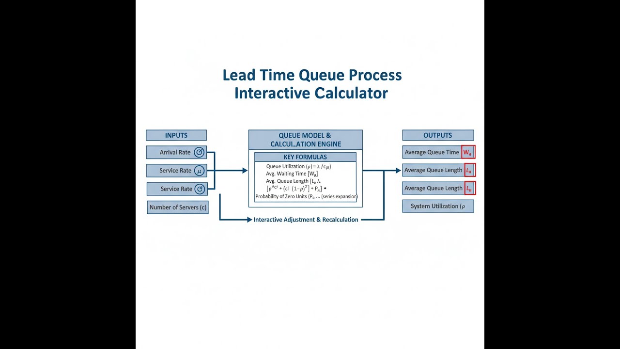
Lead Time Queue Process Interactive Calculator
Visualize how queue time dominates total manufacturing lead time and see where your production efficiency is being lost. Adjust time components to understand the massive impact of waiting versus value-added processing.
TOTAL LEAD TIME
8.0 hrs
PROCESS EFFICIENCY
25.0%
QUEUE TIME RATIO
50.0%
VALUE-ADDED TIME
2.0 hrs
FIRGELLI Automations — Interactive Engineering Calculators
Equations & Formulas
Use the formula below to calculate total lead time.
Total Lead Time
LTtotal = Tqueue + Tsetup + Tprocess + Tmove + Tinspection
Where:
LTtotal = Total lead time (hours)
Tqueue = Queue or wait time (hours)
Tsetup = Setup or changeover time (hours)
Tprocess = Processing or run time (hours)
Tmove = Transportation or move time (hours)
Tinspection = Inspection or quality check time (hours)
Use the formula below to calculate process efficiency.
Process Efficiency
ηprocess = (Tprocess / LTtotal) × 100%
Where:
ηprocess = Process efficiency (percentage)
Tprocess = Value-added processing time (hours)
LTtotal = Total lead time (hours)
Use the formula below to calculate throughput time for a batch.
Throughput Time for Batch Processing
TTbatch = Tsetup + (n × Tunit)
Where:
TTbatch = Total throughput time for batch (hours)
Tsetup = Setup time per batch (hours)
n = Number of units in batch
Tunit = Processing time per unit (hours)
Use the formula below to calculate WIP inventory using Little's Law.
WIP Inventory (Little's Law)
WIP = λ × LT
Where:
WIP = Work-in-process inventory (units)
λ = Throughput rate (units/hour)
LT = Lead time through system (hours)
Use the formula below to calculate cycle time from demand rate.
Cycle Time (Takt Time)
CT = 1 / Drate
Where:
CT = Cycle time (hours/unit)
Drate = Customer demand rate (units/hour)
Use the formula below to calculate queue time ratio.
Queue Time Ratio
QR = (Tqueue / LTtotal) × 100%
Where:
QR = Queue time ratio (percentage)
Tqueue = Queue or wait time (hours)
LTtotal = Total lead time (hours)
Simple Example
A part moves through a machining cell with these time components:
- Queue time: 4 hours
- Setup time: 1 hour
- Process time: 2 hours
- Move time: 0.5 hours
- Inspection time: 0.5 hours
Total lead time = 4 + 1 + 2 + 0.5 + 0.5 = 8 hours. Process efficiency = (2 / 8) × 100 = 25% — right at the lower bound of good manufacturing performance.
Theory & Engineering Applications
Fundamental Principles of Lead Time Analysis
Lead time represents the total elapsed time from the initiation of a production order until the completion and delivery of the finished product. In manufacturing environments, lead time comprises both value-added activities (processing) and non-value-added activities (waiting, moving, inspecting). Understanding this distinction is fundamental to lean manufacturing philosophy and forms the basis for continuous improvement initiatives across industries ranging from automotive assembly to semiconductor fabrication.
The queue time component typically dominates total lead time in most manufacturing operations, often accounting for 60-95% of the total duration. This phenomenon occurs because products spend the majority of their time waiting in queues between processing stations rather than being actively worked on. Queue formation results from capacity constraints, batch processing requirements, equipment availability limitations, and variability in both arrival rates and processing times. The relationship between queue time and system utilization follows non-linear behavior described by queuing theory, where even modest increases in utilization beyond 80% can cause exponential growth in queue lengths and wait times.
Process Efficiency and Value Stream Mapping
Process efficiency quantifies the ratio of value-added time to total lead time, providing a single metric that reveals the proportion of time a product is actually being transformed versus simply residing in the system. World-class manufacturing operations typically achieve process efficiencies between 20-30%, while traditional batch-and-queue systems often exhibit efficiencies below 5%. This stark difference highlights the massive improvement potential available through lean transformation initiatives.
Value stream mapping enables engineers to visualize material and information flow through production systems, explicitly identifying where products accumulate in queues. By mapping current state conditions including cycle times, changeover times, uptime percentages, batch sizes, and inventory levels at each process step, teams can calculate total lead time and identify the critical constraint limiting overall throughput. The future state map then establishes improvement targets by reducing batch sizes, implementing pull systems, balancing workloads, and eliminating bottlenecks.
Little's Law and WIP Inventory Relationships
Little's Law establishes a fundamental relationship in queuing systems: WIP = Throughput × Lead Time. This elegant equation reveals that work-in-process inventory levels are directly proportional to both the production rate and the time products spend in the system. For any given throughput requirement, reducing lead time directly reduces WIP inventory, freeing capital, reducing storage requirements, and decreasing the risk of obsolescence or damage.
The practical significance extends beyond simple inventory reduction. Lower WIP levels reduce the distance between process steps, making quality problems more visible and reducing the quantity of defective parts produced before detection. Manufacturing systems operating with days or weeks of WIP buffer stock can continue producing defects for extended periods before discovery, while lean systems with hours of WIP provide rapid feedback enabling immediate corrective action. This relationship fundamentally changes the economics of quality management and continuous improvement.
Batch Processing and Economic Trade-offs
Batch processing introduces complex trade-offs between setup efficiency and flow velocity. Larger batches amortize setup time over more units, reducing per-unit setup cost but increasing throughput time and WIP inventory. The classical economic order quantity (EOQ) model balances setup costs against holding costs, but this traditional approach often undervalues the hidden costs of extended lead times including reduced flexibility, increased obsolescence risk, and delayed customer feedback.
Modern approaches emphasize setup reduction through single-minute exchange of die (SMED) techniques, enabling economically viable small-batch or even single-piece flow. When setup times drop from hours to minutes, the optimal batch size decreases dramatically, enabling mixed-model production that better matches actual demand patterns. This transformation requires both technical improvements in tooling and fixturing design and operational discipline in standardizing changeover procedures.
Cycle Time, Takt Time, and Production Pacing
Cycle time represents the frequency at which completed units emerge from a process, while takt time represents the required production pace to meet customer demand. The relationship between these metrics determines whether a process has adequate capacity. If cycle time exceeds takt time, the process cannot meet demand and represents a bottleneck requiring capacity expansion or improvement. If cycle time is significantly faster than takt time, the process has excess capacity that might be deployed elsewhere or operated at reduced hours.
Balancing cycle times across multiple serial processes to match takt time represents a fundamental challenge in production system design. Unbalanced lines create bottlenecks where work accumulates and downstream starvation where operators wait for parts. Perfect balance is rarely achievable, but deliberate placement of buffer inventory at constraint operations can stabilize flow while focused improvement efforts work to expand bottleneck capacity.
Variability and Its Impact on Queue Formation
A non-obvious but critical insight from queuing theory is that variability in either arrival rates or processing times causes queue formation even when average utilization remains below 100%. The coefficient of variation (standard deviation divided by mean) for both inter-arrival time and service time distributions determines expected queue length and wait time. High variability systems require substantially lower average utilization to maintain acceptable queue lengths compared to low variability systems.
This relationship explains why theoretical capacity calculations often fail in practice. A workstation with 8 hours of available time per shift and 7 hours of scheduled work may still develop queues and miss delivery targets if work arrives irregularly or processing times vary significantly. Reducing variability through standardized work procedures, preventive maintenance to eliminate breakdowns, and demand smoothing through production leveling (heijunka) enables higher sustainable utilization rates while maintaining shorter queues.
Worked Example: Complete Lead Time Analysis
Scenario: A precision machining cell produces hydraulic valve bodies through a five-step process. A production engineer needs to calculate total lead time, identify improvement opportunities, and estimate the impact of proposed changes on WIP inventory levels.
Given Data:
- Queue time before machining: 8.7 hours
- Setup time for milling operation: 1.3 hours
- Actual milling time: 2.6 hours
- Transportation to quality inspection: 0.4 hours
- Inspection and testing time: 0.8 hours
- Current throughput rate: 4.2 units/hour
Step 1: Calculate Total Lead Time
LTtotal = Tqueue + Tsetup + Tprocess + Tmove + Tinspection
LTtotal = 8.7 + 1.3 + 2.6 + 0.4 + 0.8 = 13.8 hours
Step 2: Calculate Value-Added vs. Non-Value-Added Time
Value-added time = Tprocess = 2.6 hours
Non-value-added time = 8.7 + 1.3 + 0.4 + 0.8 = 11.2 hours
Step 3: Calculate Process Efficiency
ηprocess = (2.6 / 13.8) × 100% = 18.84%
This indicates that only 18.84% of the total lead time involves actual value-adding transformation of the material, while 81.16% consists of waiting, setup, and movement activities.
Step 4: Calculate Queue Time Ratio
QR = (8.7 / 13.8) × 100% = 63.04%
Queue time dominates the lead time, consuming nearly two-thirds of the total duration. This identifies queue reduction as the primary improvement opportunity.
Step 5: Calculate Current WIP Inventory Using Little's Law
WIP = λ × LT = 4.2 units/hour × 13.8 hours = 57.96 ≈ 58 units
The system currently holds approximately 58 units in various stages of completion at any given time.
Step 6: Evaluate Proposed Improvement Scenario
The team proposes implementing a pull system with kanban cards limiting queue size to 2.5 hours of work. What would be the impact on WIP?
New lead time = 2.5 + 1.3 + 2.6 + 0.4 + 0.8 = 7.6 hours
New WIP = 4.2 × 7.6 = 31.92 ≈ 32 units
This represents a 45% reduction in WIP inventory (from 58 to 32 units), freeing significant floor space and reducing capital tied up in inventory.
Step 7: Calculate New Process Efficiency
New ηprocess = (2.6 / 7.6) × 100% = 34.21%
Process efficiency nearly doubles (from 18.84% to 34.21%), indicating a much leaner operation with less waste.
Engineering Insights: This analysis reveals that queue time reduction yields compound benefits: shorter lead times improve customer responsiveness, reduced WIP frees capital and floor space, and higher process efficiency indicates less waste. The constraint limiting further improvement is now the 1.3-hour setup time, suggesting that SMED techniques targeting setup reduction would generate the next wave of improvement. For additional manufacturing optimization tools, visit the engineering calculator library.
Practical Applications
Scenario: Electronics Assembly Line Optimization
Jennifer, a manufacturing engineer at a contract electronics manufacturer, notices customer complaints about 3-week lead times for custom printed circuit board assemblies. Using the lead time calculator, she maps the current state: 14.2 days in queue waiting for component availability, 0.8 days for SMT machine setup, 1.1 days for actual assembly and soldering, 0.3 days for AOI inspection, and 0.6 days for functional testing. The calculator reveals total lead time of 17.0 days with process efficiency of just 6.5%, indicating massive waste. By implementing vendor-managed inventory to reduce component queue time to 2 days and applying SMED techniques to cut setup from 0.8 to 0.2 days, she recalculates the new lead time at 4.2 days—a 75% reduction that transforms the company's competitive position and enables them to win time-sensitive prototype contracts previously going to competitors.
Scenario: Medical Device Manufacturing Capacity Planning
Marcus, a production planner for surgical instrument sterilization, must determine WIP inventory levels to support a new contract requiring 180 instrument kits per day. He enters the throughput rate of 7.5 kits/hour into the calculator along with measured lead time components: 6.8 hours in queue, 1.2 hours for cleaning and preparation, 4.5 hours for autoclave sterilization cycles, 0.5 hours for post-sterilization inspection, and 0.3 hours for packaging. The calculator computes total lead time of 13.3 hours and, using Little's Law, reveals WIP inventory of approximately 100 kits constantly in process. This calculation helps Marcus properly size sterile storage areas, plan material handling capacity, and establish buffer stock levels. When he explores reducing queue time to 3 hours through better production scheduling, the calculator shows WIP dropping to 72 kits, enabling him to justify the investment in scheduling software by quantifying the space and capital cost savings from reduced inventory.
Scenario: Automotive Stamping Press Batch Sizing
Deepak, an industrial engineer at a tier-2 automotive supplier, evaluates optimal batch sizes for door panel stamping. Current practice runs 500-piece batches with 3.2-hour die changeovers. Using the throughput calculator with setup time of 3.2 hours, per-unit cycle time of 0.067 hours (4 minutes), and batch size of 500, he calculates total batch throughput time of 36.7 hours. He then models smaller batches: at 200 pieces, throughput drops to 16.6 hours; at 100 pieces, to 9.9 hours. While per-unit costs increase slightly with smaller batches due to more frequent setups, lead time improvements enable just-in-time delivery matching the assembly plant's daily schedule variations. Deepak uses the calculator to find the sweet spot at 150-piece batches (13.25 hours throughput), balancing economic efficiency with the flexibility needed to respond to engineering changes and demand fluctuations without accumulating obsolete inventory.
Frequently Asked Questions
▼ What is the difference between lead time and cycle time in manufacturing?
▼ Why does queue time dominate total lead time in most manufacturing systems?
▼ How does process efficiency below 25% affect manufacturing competitiveness?
▼ What is Little's Law and how does it apply to production planning?
▼ How do you determine the optimal batch size balancing setup costs and lead time?
▼ What role does variability play in queue formation and how can it be reduced?
Free Engineering Calculators
Explore our complete library of free engineering and physics calculators.
Browse All Calculators →🔗 Explore More Free Engineering Calculators
About the Author
Robbie Dickson — Chief Engineer & Founder, FIRGELLI Automations
Robbie Dickson brings over two decades of engineering expertise to FIRGELLI Automations. With a distinguished career at Rolls-Royce, BMW, and Ford, he has deep expertise in mechanical systems, actuator technology, and precision engineering.
Need to implement these calculations?
Explore the precision-engineered motion control solutions used by top engineers.


