Resonant Frequency LC Interactive Calculator

The Resonant Frequency LC Calculator determines the natural oscillation frequency of LC circuits — fundamental building blocks in radio transmitters, receivers, filters, and oscillators. At resonance, inductive and capacitive reactances cancel, creating unique impedance conditions essential for RF design, power electronics, and signal processing applications across telecommunications, medical devices, and precision instrumentation.

📐 Browse all free engineering calculators

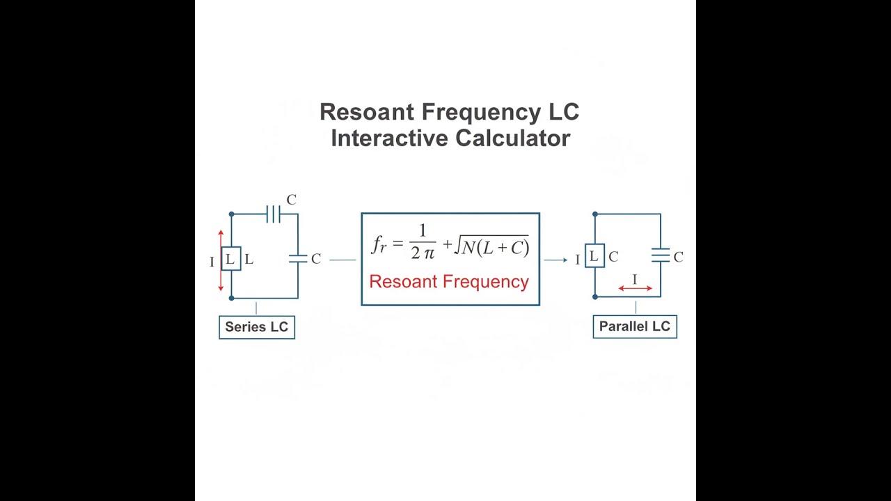
LC Circuit Diagram

Resonant Frequency Calculator

Resonance Equations

Theory & Practical Applications

Fundamental Physics of LC Resonance

LC resonance represents one of nature's most elegant energy exchanges: electromagnetic oscillation between electric and magnetic fields. When alternating current flows through an inductor, energy stores in the magnetic field surrounding the coil. This energy then transfers to the capacitor as an electric field between its plates. The cycle repeats indefinitely in an ideal lossless system, creating sustained oscillation at a specific natural frequency determined solely by the circuit's inductance and capacitance values.

The resonant frequency equation f₀ = 1/(2π√LC) emerges from setting inductive reactance X_L = 2πfL equal to capacitive reactance X_C = 1/(2πfC). At this unique frequency, the reactive impedances are equal in magnitude but opposite in phase, resulting in perfect cancellation. For series LC circuits, this produces minimum impedance limited only by parasitic resistance. For parallel LC circuits, it creates maximum impedance — a characteristic exploited in tank circuits and selective filters throughout RF engineering.

A critical non-obvious consideration often overlooked in introductory treatments: component self-resonance. Real inductors possess parasitic capacitance between windings, while real capacitors exhibit series inductance in their leads and plates. Every physical component therefore has its own self-resonant frequency where these parasitics dominate. Attempting to use a 10 μH inductor with 2 pF of parasitic capacitance at 300 MHz will fail catastrophically because the inductor's self-resonance at 356 MHz makes it behave capacitively at the design frequency. Professional RF designers select components with self-resonant frequencies at least 3-5 times higher than the operating frequency to maintain predictable behavior.

Quality Factor: The Measure of Selectivity

The quality factor Q = √(L/C)/R quantifies how sharply a resonant circuit responds to its resonant frequency versus nearby frequencies. High-Q circuits (Q > 100) exhibit narrow bandwidth and steep skirts — ideal for precision frequency selection in radio receivers. Low-Q circuits (Q < 10) provide broad bandwidth suitable for wideband matching networks and power transfer applications. The relationship Q = f₀/BW directly connects selectivity to bandwidth, where BW represents the frequency span between half-power (-3 dB) points.

In practical designs, achieving high Q requires minimizing resistance. This explains why RF inductors use thick silver-plated wire wound on low-loss ceramic forms, and why high-frequency capacitors employ specialized low-ESR (equivalent series resistance) dielectrics. Temperature-compensating capacitors (NPO/C0G types) maintain stable Q across temperature ranges, critical for precision oscillators and filters where frequency drift degrades performance. The design constraint becomes particularly severe in microwave circuits where even PCB trace resistance significantly impacts Q.

Series vs. Parallel Resonance: Dual Personalities

Series and parallel LC circuits exhibit opposite impedance characteristics at resonance, making them suited for different applications. Series resonant circuits present minimum impedance (just R) at f₀, allowing maximum current flow — the basis for series-tuned traps that short specific frequencies to ground. The voltage across the capacitor or inductor at resonance equals Q times the applied voltage, creating voltage magnification that can damage components if Q exceeds safe limits. A 12V input with Q=50 produces 600V across the capacitor — requiring components rated for this stress.

Parallel resonant circuits present maximum impedance at f₀, ideally approaching infinity but limited practically to Z_max = L/(CR) by resistive losses. This high impedance blocks current at resonance while allowing other frequencies to pass, forming the foundation of parallel-tuned bandpass filters. Tank circuits in oscillators exploit this behavior: the parallel LC presents high impedance at f₀, providing maximum gain and positive feedback at the desired oscillation frequency while attenuating harmonics.

Applications Across Engineering Disciplines

LC resonators pervade modern technology in forms ranging from microscopic MEMS oscillators to room-sized antenna tuning networks. In telecommunications, every radio receiver contains multiple LC filters defining channel selectivity — typically 7-10 resonators in a superheterodyne receiver's IF strip. The 455 kHz IF transformer in AM radios uses precisely matched 100 μH coils with specific core permeability to achieve consistent bandwidth across production. Crystal replacements for LC oscillators offer higher Q (10,000-100,000 versus 20-200 for LC), but LC circuits remain dominant where tuning range matters more than absolute stability.

Induction heating systems use LC resonance to achieve efficient power transfer at frequencies from 3 kHz (forge heating) to 400 kHz (induction cooktops). The workpiece forms the resistive element in a series resonant circuit, while the LC tank operates at resonance to minimize reactive power draw. A typical 3.5 kW cooktop uses a 140 μH coil with 140 nF capacitance, resonating at 22 kHz. The high circulating currents (150-300 A) despite modest input power require water-cooled Litz wire construction.

Medical MRI scanners employ massive LC circuits tuned to the Larmor frequency corresponding to the magnetic field strength — 127.7 MHz for a 3 Tesla system. The body coil inductance of approximately 2.8 μH requires 560 pF of distributed capacitance to achieve resonance. Q factors of 200-400 are essential for achieving the sensitivity needed to detect weak nuclear magnetic resonance signals. Temperature stabilization maintains frequency accuracy to within ±100 Hz across varying patient loads.

Wireless power transfer systems, from Qi smartphone chargers to industrial conveyor systems, rely on loosely-coupled LC resonators. The transmitter coil resonates at 100-200 kHz (Qi standard specifies 87-205 kHz), with typical values of L=15 μH and C=220 nF for 125 kHz operation. The receiver coil must match this frequency precisely despite variations in spacing and alignment. Modern designs use adaptive tuning with switched capacitor banks to maintain resonance across the ±5 mm coupling distance tolerance.

Worked Example: FM Radio Antenna Tuner Design

Design a tunable LC circuit for an FM radio front-end that covers the commercial FM broadcast band (87.5-108 MHz) with adequate selectivity to reject adjacent channels spaced 200 kHz apart.

Step 1: Determine Component Values for Mid-Band

Target mid-band frequency: f₀ = 97.75 MHz

Select a practical variable capacitor: C = 8-45 pF (common RF tuning capacitor range)

Using C = 25 pF (mid-range) at center frequency:

L = 1 / [(2πf₀)² × C] = 1 / [(2π × 97.75×10⁶)² × 25×10⁻¹²]

L = 1 / [(6.142×10⁸)² × 25×10⁻¹²] = 1 / (9.437×10¹⁵) = 106 nH

Step 2: Verify Tuning Range

At minimum capacitance (8 pF):

f_max = 1 / (2π√(106×10⁻⁹ × 8×10⁻¹²)) = 173.0 MHz (exceeds required 108 MHz)

At maximum capacitance (45 pF):

f_min = 1 / (2π√(106×10⁻⁹ × 45×10⁻¹²)) = 73.1 MHz (below required 87.5 MHz)

The 8-45 pF range is too wide. Recalculate using C = 15-30 pF range:

At C = 15 pF: f = 126.5 MHz
At C = 30 pF: f = 89.4 MHz

This range (89.4-126.5 MHz) covers the FM band with margin. Exact inductance becomes:

L = 1 / [(2π × 97.75×10⁶)² × 22.5×10⁻¹²] = 118 nH

Step 3: Calculate Required Q for Selectivity

For 200 kHz channel spacing with adequate rejection, bandwidth should be ≤100 kHz:

Q = f₀ / BW = 97.75×10⁶ / 100×10³ = 977.5

This Q is unrealistically high for a simple LC circuit. Practical approach uses Q ≈ 50-100 in the front-end, followed by high-Q ceramic filters in the IF stage for selectivity.

For Q = 80, maximum allowable series resistance:

X₀ = √(L/C) = √(118×10⁻⁹ / 22.5×10⁻¹²) = 72.4 Ω

R_max = X₀ / Q = 72.4 / 80 = 0.905 Ω

Step 4: Component Selection and Parasitic Effects

Air-core inductor wound with 18 AWG wire: 6 turns, 8 mm diameter, 10 mm length gives approximately 118 nH with Q ≈ 90 at 100 MHz. The self-resonant frequency (limited by inter-turn capacitance ≈ 0.8 pF) occurs at approximately 430 MHz — safely above operating range.

Silver-mica or NPO ceramic variable capacitor with low-loss dielectric maintains Q > 1000 at 100 MHz, making the inductor the limiting factor. Total circuit Q = 85 (slightly better than target due to low capacitor losses).

Bandwidth at 97.75 MHz: BW = 97.75×10⁶ / 85 = 1.15 MHz

This provides moderate selectivity while maintaining tunable bandwidth. The subsequent IF strip at 10.7 MHz employs ceramic filters with Q > 1000 for the required adjacent channel rejection.

Step 5: Temperature Stability Analysis

Inductance temperature coefficient: +30 ppm/°C (air-core)
Capacitance temperature coefficient: -30 ppm/°C (NPO ceramic, specified)

Combined frequency drift: Since f ∝ 1/√LC, temperature coefficients partially cancel:

Δf/f ≈ -½[(ΔL/L) + (ΔC/C)] = -½[(30-30) ppm/°C] = 0 ppm/°C (theoretical)

In practice, achieving perfect compensation requires careful component selection and matching. Residual drift of ±5 ppm/°C is typical, producing ±489 Hz shift at 97.75 MHz over a 0-50°C temperature range — acceptable for FM broadcast applications where AFC (automatic frequency control) corrects drift.

For more detailed engineering calculations and specialized resonant circuit designs, visit the complete engineering calculator library.

Frequently Asked Questions