Hair Diffraction Interactive Calculator

This interactive calculator determines the diameter of a human hair using single-slit diffraction principles. By measuring the distance between diffraction minima when laser light passes through a strand of hair, this tool calculates hair thickness with micrometer precision—a classic demonstration of wave optics used in physics education, forensic analysis, and materials characterization laboratories worldwide.

📐 Browse all free engineering calculators

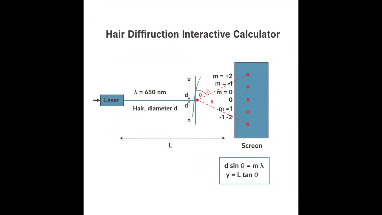
Diffraction Setup Diagram

Hair Diffraction Calculator

Governing Equations

Theory & Practical Applications

Physical Basis of Single-Slit Diffraction

When coherent light encounters an obstruction comparable in size to its wavelength, diffraction produces an interference pattern fundamentally different from geometric shadow predictions. A human hair acts as a single-slit diffractor—though technically the inverse (opaque obstacle rather than aperture), Babinet's principle ensures the diffraction patterns are identical except at θ = 0. Each point across the hair's width acts as a secondary wave source according to Huygens' principle, with path differences creating constructive and destructive interference.

The critical insight that separates expert analysis from superficial understanding: diffraction minima occur when the slit width creates exactly m whole wavelengths of path difference between rays from opposite edges, causing complete destructive interference. This differs fundamentally from double-slit interference, where minima occur at half-wavelength path differences. For hair diffraction at the first minimum (m=1), a ray from the top edge and a ray from the center travel paths differing by λ/2, while a ray from just below the top and one from just below center also differ by λ/2—these pairs destructively interfere across the entire aperture width. This zone-pairing argument, absent from most introductory treatments, explains why the condition is d sin θ = mλ rather than the double-slit formula.

Small Angle Approximation Validity

The linear fringe spacing formula y = mλL/d employs three sequential approximations that accumulate error at larger angles. First, tan θ ≈ θ assumes the screen distance greatly exceeds fringe displacement (L ≫ y), introducing ~0.1% error at θ = 5° but 1.5% at θ = 15°. Second, sin θ ≈ θ approximates the diffraction condition itself, with similar error scaling. Third, measuring y as a straight-line distance rather than arc length on a spherical wavefront adds negligible error for typical setups but becomes significant in extreme wide-angle configurations.

Practicing optical engineers recognize that cumulative error exceeds 5% beyond θ ≈ 10°, necessitating exact trigonometric treatment. For a 65 μm hair and 650 nm red laser at L = 1.5 m, the first minimum appears at y = 15.0 mm using the approximate formula, versus 14.97 mm from exact calculation—acceptable for educational demonstrations but insufficient for precision measurement. Beyond m = 3 for this configuration (θ = 17.2°), errors exceed 10%, and fringe visibility degrades due to intensity fall-off following the sinc² function envelope.

Wavelength Dependence and Color Effects

Hair diffraction provides elegant wavelength measurement because fringe spacing scales linearly with λ. White light produces separated color spectra at each order, with violet fringes (λ ≈ 400 nm) appearing 39% closer to the central maximum than red fringes (λ ≈ 650 nm). This dispersion enables spectroscopic analysis: unknown laser wavelengths can be determined by measuring fringe positions against a calibrated hair standard. The technique historically measured mercury emission lines (435.8 nm, 546.1 nm, 579.1 nm) with ±2 nm precision using mechanical micrometer stages.

However, practical white-light observations reveal a critical limitation: spectral overlap beyond the first order. The second-order violet minimum (m=2, λ=400 nm) appears at the same angular position as the first-order minimum of a 800 nm wavelength that doesn't exist in the visible spectrum, but third-order violet (m=3) coincides with second-order green (m=2, λ=600 nm). This overlap smears higher-order fringes into a continuous spectrum unsuitable for precise measurement, restricting quantitative work to first-order analysis with monochromatic sources.

Applications in Forensic Science

Forensic hair analysis employs diffraction-based diameter measurement as a non-destructive identification technique. Human head hair ranges from 40-120 μm depending on ethnicity (Asian hair averages 80-120 μm, Caucasian 50-70 μm, African 40-60 μm), while body hair exhibits distinct diameter profiles. A 632.8 nm HeNe laser directed through a hair sample 1.2 m from a screen produces first-order fringes at 9.5 mm for 80 μm hair versus 15.8 mm for 48 μm hair—easily distinguishable with millimeter-scale measurements.

Crime laboratories combine diffraction data with microscopic scale pattern analysis and medullary index measurements. The technique's advantage over direct microscopy: no sample preparation, no mounting media, and no physical contact that might transfer contaminating fibers. Cross-sectional shape affects results—elliptical hairs produce asymmetric fringe patterns where orthogonal diffraction measurements yield major and minor axis diameters. Advanced forensic protocols measure at multiple orientations, rotating the hair through 90° increments to characterize cross-sectional geometry rather than assuming circular symmetry.

Industrial Quality Control Applications

Textile manufacturing uses laser diffraction gauges for real-time fiber diameter monitoring during extrusion processes. Synthetic fibers require ±2 μm tolerance across kilometer production runs, achievable only through continuous non-contact measurement. A production line extruding 65 μm polyester fiber at 50 m/min employs a 520 nm green laser diffraction sensor sampling at 1 kHz, detecting diameter variations from tension fluctuations, temperature drift, or polymer viscosity changes within milliseconds.

The system exploits the inverse relationship between diameter and fringe spacing: a 3% diameter reduction causes a 3% fringe spacing increase, detected as a 0.5 mm shift in first-order position. CCD linear arrays positioned at the diffraction plane measure fringe centroids with 10 μm spatial resolution, translating to 0.13 μm diameter resolution at 1.5 m optical path length. Feedback controllers adjust extrusion rate and die temperature within 200 ms to maintain specification, preventing kilometers of out-of-tolerance production that would occur with periodic sampling-based quality control.

Worked Example: Complete Hair Measurement Procedure

Scenario: A materials laboratory needs to characterize a new biocompatible fiber for surgical sutures. The fiber is specified at 73.0 μm nominal diameter with ±3 μm tolerance. A quality control technician uses a 638 nm red diode laser and a measurement screen positioned exactly 1.850 m from the fiber mount. The technician measures the distance from the central bright fringe to the first dark fringe on both sides, recording 16.3 mm to the right and 16.1 mm to the left.

Part A - Calculate Fiber Diameter from Each Measurement:

For the right-side measurement (y₁ = 16.3 mm = 0.0163 m):
Using d = (m λ L) / y with m = 1, λ = 638 × 10⁻⁹ m, L = 1.850 m:
d₁ = (1 × 638 × 10⁻⁹ × 1.850) / 0.0163
d₁ = (1.1803 × 10⁻⁶) / 0.0163
d₁ = 7.242 × 10⁻⁵ m = 72.42 μm

For the left-side measurement (y₂ = 16.1 mm = 0.0161 m):
d₂ = (1 × 638 × 10⁻⁹ × 1.850) / 0.0161
d₂ = (1.1803 × 10⁻⁶) / 0.0161
d₂ = 7.331 × 10⁻⁵ m = 73.31 μm

Part B - Assess Measurement Quality:

Average diameter: d_avg = (72.42 + 73.31) / 2 = 72.87 μm
Standard deviation: σ = 0.63 μm
Measurement uncertainty: ±2σ = ±1.26 μm (95% confidence)

Asymmetry between left and right measurements (0.89 μm difference) suggests slight fiber tilt or non-circular cross-section. The left-right average compensates for minor alignment errors, a standard practice in precision diffraction measurement.

Part C - Verify Small Angle Approximation Validity:

Using average y = 16.2 mm:
tan θ = y / L = 0.0162 / 1.850 = 0.008757
θ = arctan(0.008757) = 0.5017° = 0.00876 rad

For small angle check, sin θ should equal θ within 1%:
sin(0.5017°) = 0.008757
Error = |0.008757 - 0.00876| / 0.00876 = 0.03% — excellent validity

Part D - Calculate Higher Order Positions for Pattern Verification:

Second-order minimum (m = 2):
y₂ = (2 × 638 × 10⁻⁹ × 1.850) / (7.287 × 10⁻⁵)
y₂ = 32.4 mm

Third-order minimum (m = 3):
y₃ = (3 × 638 × 10⁻⁹ × 1.850) / (7.287 × 10⁻⁵)
y₃ = 48.6 mm

These predictions allow the technician to verify the measurement by checking that additional minima appear at the calculated positions. Observing all three orders confirms the fiber is uniform along the illuminated length and validates the measurement methodology.

Part E - Quality Control Decision:

Measured diameter: 72.87 ± 1.26 μm
Specification: 73.0 ± 3.0 μm (70.0 - 76.0 μm acceptable range)
Result: PASS — fiber meets specification with comfortable margin

The measurement demonstrates 1.7% precision (±1.26 μm on 72.87 μm), significantly better than the 4.1% tolerance window. This precision suffices for surgical suture applications where diameter uniformity affects knot strength and tissue trauma. The technique's non-contact nature preserves sterile packaging integrity, unlike micrometer measurements requiring sample extraction.

Intensity Distribution and Fringe Visibility

Beyond geometric fringe positions, diffraction intensity follows I(θ) = I₀ [sin(β)/β]² where β = (πd sin θ)/λ. This sinc² function creates the characteristic pattern: a bright central maximum containing 90.3% of total diffracted power, with rapidly diminishing side maxima. The first side maximum reaches only 4.7% of central intensity, explaining why high-order fringes become difficult to observe in practice despite geometric predictions suggesting their existence.

Fringe contrast degrades with increasing order due to three mechanisms: sinc² envelope decay, finite laser coherence length, and polychromatic line width. Even "monochromatic" laser diodes exhibit 0.1-2 nm spectral width, causing fifth-order fringes for 650 nm light to blur by ±0.8% of their spacing—approaching the fringe width itself. Professional measurements therefore restrict analysis to orders where fringe visibility V = (I_max - I_min)/(I_max + I_min) exceeds 0.3, typically limiting practical work to m ≤ 4 for hair-diameter objects.

Frequently Asked Questions