Camera Exposure Aperture Iso Interactive Calculator

The Camera Exposure Triangle Calculator provides precise calculations for the fundamental relationship between aperture (f-stop), shutter speed, and ISO sensitivity that determines photographic exposure. This interactive tool solves exposure equations across multiple scenarios, enabling photographers, cinematographers, and optical engineers to optimize image capture settings for specific lighting conditions, motion requirements, and depth of field objectives while maintaining equivalent exposure values (EV).

📐 Browse all free engineering calculators

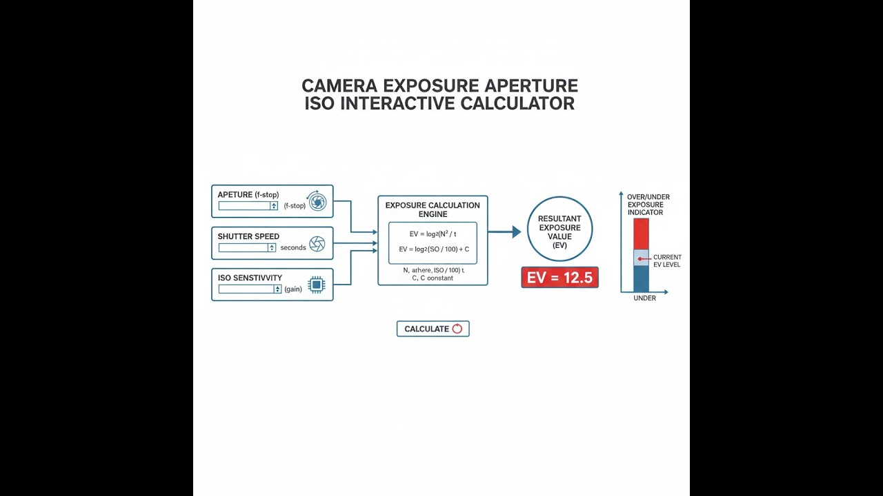
Exposure Triangle Diagram

Camera Exposure Calculator

Exposure Equations & Formulas

Theory & Engineering Applications

The exposure triangle represents one of the fundamental engineering trade-offs in optical imaging systems. Unlike purely mathematical relationships, photographic exposure involves complex interactions between optical physics, sensor technology, and signal processing that create practical limitations not evident from equations alone. The relationship between aperture, shutter speed, and ISO sensitivity determines not only the quantity of light reaching the sensor but also critical image characteristics including depth of field, motion blur, and signal-to-noise ratio.

The Physics of Aperture and Light Transmission

The f-number (N) represents the ratio of focal length to entrance pupil diameter, making it fundamentally a geometric relationship: N = f/D. What makes this relationship non-intuitive is that light transmission scales with the square of the f-number. Moving from f/2.8 to f/4 reduces the aperture diameter by approximately 1.4×, but reduces light transmission by 2× (one stop) because the aperture area decreases by the square of the diameter ratio. This quadratic relationship means that extremely wide apertures (f/1.4, f/1.2) transmit dramatically more light than moderate apertures — f/1.4 transmits 4× more light than f/2.8, not 2× as linear intuition might suggest.

The engineering challenge with wide apertures extends beyond simple light gathering. Lens aberrations become progressively more difficult to correct at wider apertures because off-axis light rays strike lens elements at more extreme angles. Spherical aberration, coma, and astigmatism all increase with aperture diameter, requiring increasingly complex lens designs with aspherical elements and specialized optical coatings. This explains why f/1.4 prime lenses cost significantly more than f/2.8 zooms ��� the optical engineering complexity grows exponentially with aperture width.

Shutter Speed and Temporal Integration

Shutter speed represents the temporal integration period during which photons accumulate on the sensor. The relationship between shutter speed and exposure is strictly linear — halving the shutter speed from 1/125 to 1/250 second precisely halves the total light captured. However, the practical implications extend well beyond exposure control. Mechanical focal-plane shutters use two curtains traveling across the sensor, creating a moving slit at very high speeds. At 1/8000 second, the second curtain begins closing before the first curtain fully opens, creating a narrow vertical slit that sweeps across the frame. This generates the notorious "rolling shutter" effect with flash photography, where part of the frame appears dark because the flash fired while part of the sensor was covered by a shutter curtain.

Electronic shutters in modern cameras eliminate mechanical limitations but introduce different artifacts. Global shutter sensors read all pixels simultaneously, but most consumer cameras use rolling shutters that read pixels row-by-row. At very fast shutter speeds (1/8000 to 1/32000 second electronic), fast-moving subjects can exhibit spatial distortion where different parts of the subject are captured at slightly different times. A propeller might appear bent, or a golf club mid-swing shows impossible curvature. These temporal artifacts become significant when shutter duration approaches the time scale of subject motion.

ISO Sensitivity and Signal Amplification

Despite marketing that presents ISO as a sensor sensitivity setting, ISO in digital cameras is fundamentally an analog gain amplification applied to the sensor signal before analog-to-digital conversion. The sensor photodiodes have a fixed quantum efficiency — their ability to convert photons to electrons doesn't change with ISO setting. What changes is the amplification factor applied to the electrical signal those electrons generate. At ISO 100, the raw sensor signal receives minimal amplification. At ISO 3200, the same signal is amplified 32× (5 stops).

This amplification-based approach creates a fundamental signal-to-noise trade-off. The sensor signal contains both true image information and random electronic noise from thermal fluctuations and read noise. Amplifying the signal by 32× also amplifies the noise by 32×, degrading the signal-to-noise ratio (SNR). Modern sensors mitigate this through dual-gain architectures where high ISO settings switch to a lower-noise amplification path, and through advanced on-sensor analog-to-digital converters that minimize quantization noise. However, the fundamental physics of shot noise (Poisson noise in photon arrival) remains unavoidable — fewer photons mean higher relative noise regardless of sensor technology.

Worked Engineering Example: Wildlife Photography System Design

A wildlife photographer needs to capture birds in flight at a nature reserve. The scene has an incident light meter reading of EV 11 (typical for overcast daylight). The photographer uses a 600mm f/4 telephoto lens and needs to determine optimal exposure settings for sharp images of birds moving at 15 m/s at a distance of 20 meters.

Step 1: Calculate Required Shutter Speed for Motion Freezing

For a 600mm lens at 20m subject distance with a full-frame sensor (36mm width), the angular field of view is approximately 3.4 degrees. A bird moving at 15 m/s perpendicular to the optical axis creates angular motion of:

ω = v / d = 15 m/s / 20 m = 0.75 rad/s = 43 degrees/second

For acceptable sharpness (maximum 0.5 pixel blur on a 24-megapixel sensor with 6 μm pixels), the image motion during exposure must be less than 3 μm. With a 600mm focal length:

Angular motion limit = 3 μm / 600 mm = 5 × 10⁻⁶ radians

Maximum shutter time = 5 × 10⁻⁶ rad / 0.75 rad/s = 6.7 × 10⁻⁶ seconds

However, a more practical rule is the reciprocal rule with safety factor: t = 1 / (2 × focal_length) = 1 / 1200 second = 0.00083 seconds. For moving subjects, increase by 4× minimum: t = 1/4800 second ≈ 1/5000 second (0.0002 seconds)

Step 2: Calculate Base Exposure Settings

With EV 11 target, using the exposure equation and working backward from required shutter speed:

EV = log₂(N² / t) + log₂(S / 100)

11 = log₂(N² / 0.0002) + log₂(S / 100)

Starting with the lens wide open at f/4.0:

11 = log₂(16 / 0.0002) + log₂(S / 100)

11 = log₂(80000) + log₂(S / 100)

11 = 16.29 + log₂(S / 100)

log₂(S / 100) = -5.29

S / 100 = 2⁻⁵·²⁹ = 0.0256

S = 2.56 — This is impossibly low (below ISO 100 base).

This indicates the scene is too bright for the required shutter speed at f/4. Recalculating with stopped-down aperture at f/5.6 (one stop):

11 = log₂(31.36 / 0.0002) + log₂(S / 100)

11 = 17.29 + log₂(S / 100)

log₂(S / 100) = -6.29

S = 1.3 (still too low)

The correct approach: Accept that 1/5000 second at f/4 requires dark conditions. For EV 11, solve for achievable shutter speed at minimum ISO 100:

11 = log₂(16 / t) + log₂(100 / 100)

11 = log₂(16 / t)

2¹¹ = 16 / t

t = 16 / 2048 = 0.0078 seconds = 1/128 second

Step 3: Engineering Solution

The physics reveals the fundamental constraint: EV 11 at f/4 with ISO 100 yields 1/128 second maximum shutter speed. To achieve 1/5000 second, we need 5.3 stops more light, requiring either:

• Option A: Increase ISO to 4096 (ISO 4000, 5.3 stops above ISO 100). Settings: f/4, 1/5000s, ISO 4000. This maintains f/4 for shallow depth of field but introduces noise.
• Option B: Wait for brighter conditions (EV 16+, full sun). At EV 16: f/4, 1/5000s, ISO 100 works perfectly.
• Option C: Use f/2.8 lens (2 stops faster), allowing f/2.8, 1/5000s, ISO 1000 for better noise performance.

Real-World Selection: Professional wildlife photographers typically choose Option C (f/2.8 super-telephoto) or accept Option A with modern low-noise sensors. The calculation reveals why 600mm f/2.8 lenses cost $12,000+ — they provide the 2-stop advantage critical for action photography in variable light.

Advanced Applications in Machine Vision

Industrial machine vision systems apply exposure triangle principles with different priorities than photography. A circuit board inspection system operating at 120 frames per second requires 1/120 second maximum exposure time (0.0083s). With LED strobe illumination providing EV 14, engineers must balance aperture for depth of field against ISO noise for defect detection algorithms.

For a system detecting 0.1mm defects on a 50mm field of view, diffraction-limited resolution requires apertures no smaller than f/8. At EV 14 with t = 1/120s and N = 8:

14 = log₂(64 / 0.0083) + log₂(S / 100)

14 = 12.93 + log₂(S / 100)

S = 100 × 2^1.07 = ISO 210

Machine vision cameras typically operate at ISO 200-400 with specialized low-noise sensors optimized for this range. The exposure calculator enables engineers to rapidly determine whether proposed lighting, optics, and framerate specifications are physically compatible, often revealing the need for brighter illumination or larger sensors before hardware procurement.

More sophisticated applications include multi-exposure HDR imaging where three exposures at 2-stop intervals capture scene dynamic range exceeding 12 EV. The calculator determines the stop spacing and exposure progression needed to avoid clipping in highlights and shadows while maintaining consistent aperture for depth of field.

Practical Applications

Frequently Asked Questions